Nielsen, A. E., Kinetics of precipitation. Pergamon Press, London, 1964. Nylt, J., Sohnel, 0., Matuchova, M., Broul, M., The Kinetics of Industrial Crystallization.
Downloaded By: [HEAL-Link Consortium] At: 07:17 14 July 2008
© 1995 OPA (Overseas Publishers Association)
Chern. Eng. Comm., 1995, Vol. 136, pp. 177-199 Reprints available directly from the publisher Photocopying permitted by license only
Amsterdam B.V. Published under license by Gordon and Breach Science Publishers SA Printed in Malaysia
EVALUATION OF NUMERICAL METHODS FOR SIMULATING AN EVOLVING PARTICLE SIZE DISTRIBUTION IN GROWTH PROCESSES M. KOSTOGLOU and A.J. KARABELAS· Chemical Process Engineering Research Institute and Department of Chemical Engineering, Aristotle University of Thessaloniki, Univ. Box 455 GR 54006 Thessaloniki, Greece (Received December /6, /994)
The particle growth term renders hyperbolic the dynamic population balance equation. Problems associated with the numerical solution of hyperbolic partial differential equations with stationary grid methods are well known. Moreover in the common case of combined molecular particle growth and coagulation. the
convolution integral of the coagulation terms makes the moving grid methods computationally intractable. To cope with practical problems, this work is focused on numerical solution methods, of the population balance equation, characterized by relatively small computational cost and fair accuracy - comparable to that of relevant experimental data. For this purpose, previous work on appropriate discretization of the coagulation termsis extended forthe growth terms. Severalnumerical methods aresystematicallyevaluated and further extended. Recommendations are made concerning the best method, by taking into account the nature of the problem, the prevailing physical conditions, and the main quantity of interest; i.e. certain specific moments, or the entire size distribution KEYWORDS
Molecular particle growth
Finite differenoe methods
Population balances
INTRODUCTION Size growth of individual particles is considered here through addition of molecular, ionic or monomeric species. Simulation of such phenomena is of interest in industrial crystallization (Dirksen and Ring, 1991),aerosol dynamics (Friedlander, 1977),precipitation (Nielsen, 1967) and polymerization processes (Matsukas and GuJari, 1991). Mathematical formulation is simple; yet obtaining solutions in many cases of practical interest is not a trivial matter. Particle size reduction through reverse mechanisms [e.g. droplet evaporation (Tsang and Huang, 1990) and particle dissolution (LeBlank and Fogler, 1987)] is formulated in a similar manner. This reduction, however, is mathematicallya more complex problem since the population number is not conserved due to gradual particle disappearance. In many practical cases there are, of course, simultaneously occurring particle growth and diminution processes, as for example in Ostwald ripening (Tsang and Brock, 1986). Size growth through coagulation can be ignored only when particle-particle collision frequency is negligible compared to that of molecule-particle encounters. In that case
• Author for correspondence. 177
Downloaded By: [HEAL-Link Consortium] At: 07:17 14 July 2008
M. KOSTOGLOU AND A. J. KARABELAS
178
the equations describing particle concentration are written as
(I) where Wi = 0 for j = I,. " , j* - 1. For j < j* there are no particles but molecular clusters. Henceforth, the elementary species (molecules, ions, monomers, other) will be referred to as monomers for simplicity. Equation (I) can be recast as follows
af(x, t) aG(x)f(x, t) -a-t-= ax
x. a 2 G(x)f(x, t)
2"
ax 2
(2)
by considering a continuous distribution f(jx., t) = Wi/X., and a growth rate function (kernel) G(ix.) = k,w,x., where x' = ix; and x. is the monomer volume. The third term in Eq. (2) may be neglected if (Ramabhadran et al., 1976) f(2)(X', t)
.
I'" (x', t) «I This condition is satisfied in almost all problems of practical interest (Ramabhadran et al., 1976). In the relatively recent literature on crystallization, there is a tendency to introduce in Eq. (2) the so-called "growth rate dispersion" terms in efforts to reconcile predictions with experimental data (Tavare, 1985). This approach is phenomenological, accounting for possible macroscopic variations of growth rate, and bears no relation to the basic mechanism of particle growth via molecular diffusion. Two kinds of size growth problems can be recognized, depending on initial and boundary conditions. One refers to an initial value problem if a given size distribution evolves through individual particle growth; or to a source problem, if molecules are produced by a chemical reaction with a tendency to nucleate. In this case a hybrid (discrete - continuous) type of an approach may be used; i.e. discrete for the small "agglomerates" (particles or molecular clusters) and continuous for larger units (Gel bard and Seinfeld, 1979a). Alternatively, the theory of homogeneous nucleation may be employed with the boundary condition set at the critical nuclei size (Nyvlt et al., 1985), through a series of assumptions. TABLE 1 Typical particle growth rate functions of the form G(x) = G xl 9
o If3 2f3 I
Mechanism
Reaction controlled process with fixed number of surface sites Diffusion controlling Surface reaction controlling Volume reaction controlling
Example Linear chain polymers (Matsukas and Gulari, 1991) Aerosols, precipitation
Crystallization Aerosols (Gelbard and Seinfeld 1979a). Porous particle totally permeable to monomers
(Matsukas an Gulari, 1991)
Downloaded By: [HEAL-Link Consortium] At: 07:17 14 July 2008
EVALUATING PARTICLE SIZE DISTRIBUTION
179
A common form of the growth function is G(x) = G x 9 • Table I includes typical exponent values, corresponding to several basic growth mechanisms, which cover the range zero to unity. For particles of fractal geometry the exponent 9 is again between oand 1. For a combination of more than one basic processes, the rate function is more complicated although the slope dlog [G(x)]/dlog(x) is everywhere in between the slopes of the constituent mechanisms. Some characteristics of the growth function are noteworthy. Strong G(x) functions lead to particles of infinite size within a finite time period. It can be shown that the condition to avoid this is lim [x/G(x)] ;
/.
I-"'"[~
5
10
-- ''oj 15
... 20
-\ 25
class
FIGURE I Particle size distribution computed numerically (FOFD) for monodisperse initial distribution and two growth kernels and time scales. Vertical lines show the location oftheexact monodisperse solutions.
Downloaded By: [HEAL-Link Consortium] At: 07:17 14 July 2008
186
M. KOSTOGLOU AND A. J. KARABELAS
expecting to have the aforementioned benefits. However, this operation is ineffective, since the system of finite difference equations is of similar form regardless of the independent variable employed. Figure 2 includes results for two of the most common kernels, those with exponents 1/3 and 2/3. For exponent 1/3 (diffusion limited process), the numerical solution displays the same general behaviour as that of constant kernel but with "phase lag" equal to one and a slightly broader particle size distribution. For exponent 2/3 (reaction limited mechanism) there is noticeable diffusion between the two times of computations, which is, however, much smaller compared to the case oflinear kernel. The "lag" ofthe numerical solution (compared to the exact one) is 1for r = 64 and 2 for r = 106 for the kernel with g = 2/3. For a linear kernel the respective lag is 2 and 7. In Figure 3 typical results are presented for the category of problems involving an initial distribution of exponential type. A computation time is selected corresponding to
0.40
(\
0.35
- - .=113 ,=11.5 .=1/3 '=15000 .=1/3 ,=9
0.30 \
0.25
c
1=1/3 ~=297 \
I
- 0.20 I
'\
f
0.10 0.05 ~ 0.00
/,)
0
,.1' /.
10
5
1
:'1 ". \ :' 1 . \ :' I ".\ ;' I '.\
f I
0.15
1\
15
\.
, 20
25
class
FIGURE 2 Particle size distribution computed numerically (FOFD) for exponential initial distribution and two growth kernels and lime scales.Vertical lines show the location of the exact monodisperse solutions.
0.70 - - 1=0 ~=1 Dum.
0.60
1=0 ~=l nat. 1=1 -.:=108(2) Dum.
0.50
, .. I '1=101(1) end
c
-
0.40 0.30 0.20 0.10 0.00 0
2
4
8
8
10
12
14
18
class
FIGURE 3 Comparison between numerical (FOFD) and analytical solution of growth equation for exponential initial distribution; constant and linear kernel.
Downloaded By: [HEAL-Link Consortium] At: 07:17 14 July 2008
EVALUATING PARTICLE SIZE DISTRIBUTION
187
doubling of the system mass. The trend appears to be reversed here compared to the previous category. For a constant kernel the numerical solution yields (erroneously) a broader distribution, lagging behind the exact one. For a linear kernel the finite difference solution is much more representative of the true distribution. The performance of the first order finite differences is examined next as regards the moments of the distribution. A measure of that performance is the ratio R of numerical over exact value of a moment. For the monodisperse initial distribution, employed here, the exact value of moments is obtained (Williams, 1983) as follows M k = [1
+ (1 -
g)r](k/t-.)
9-+p+qr=O j
r
i= 1
(15a)
ii) Mass conservation
dM -d =
f'" G(x)F(x,r)d.x=>-d ~ d (h 1 + r L -2-Si-lnj )
to.
=
L h
j=
I
r
(I + r)
Gin,=> -
2r
i=l
(m+p+q)= 1
(15b)
Downloaded By: [HEAL-Link Consortium] At: 07:17 14 July 2008
EVALUATING PARTICLE SIZE DISTRIBUTION
191
iii) Conservation of n-th order moment
ddMn=n r
roo Xn-1G(X)F(x,T)dx=dd
Jo
t
h
L G;ni=mr" i= 1 r: I
=n
-1
(.t
I-n
+p+qr.
K nS7_l ni)
1=1
=
nrG~n-l) 1
K n s7- , Gi
=B
(15c)
I _
K =-----;-n
n+ I
By solving the system of Equations (15) one obtains 2
n
m= ( 2 r (1 - r- ) +B (1 - r)) -I I +r D n-r") p= (2r(r+B(r-~)).!I +r r D 2r(rn- I - - : I q= ( +B - - I I +r r D
(I )) 1
(16a)
(16b)
(16c)
D=r-n-rn+r"-I-rl-n+r-r-I For a generalized kernel G(x) = Gx9 B=
nr(n + 1)(r"+9 - 1)(1 + g) .,.--"...i-;----=',..'-,,.-;-,:---='-;;.;,.. (r n + 1 _ I)(r ' +9 - l)(n + g)
As already discussed in the case of first order finite differences, for exponent g = I, exact predictions of all moments can be made whereas for g = 0 only of moments n = 0, 1,2. Additionally, using the transformation z = [G(x)] - I d i: one can compute exactly the quantities
J
1"
ZF(X,T)dx
and
L"
z 2F(x,T)dx
For kernels G(x) = G x 9, these quantities correspond to moments M(1-9) and M 2(1-9) respectively. In particular, g = 2/3 represents the case already treated by Hounslow et al. (1988). A serious drawback of the above method is the dispersion problem appearing with increasing time. Oscillations actually commence after vanishing of the first class. By automatically setting negative values equal to zero one can take care of the problem. However, this treatment seriously restricts the use of integrators with self-adjusting step and predetermined accuracy. Table 5 shows the short time period over which stable computations can be carried out with such integrators. This time T indicates the onset of oscillations, for various exponent values. Thus for longer times one should use an integration technique with constant step size. By employing this approach in the case of surface reaction controlled growth, Hounslow (1988) manages to move foreward in time considerably.
Downloaded By: [HEAL-Link Consortium] At: 07:17 14 July 2008
M. KOSTOGLOU AND A. J. KARABELAS
192
TABLE 5 Maximum integration time
against growth
'flit
exponent 9 fm
9
0.5 0.6 0.7 0.8 0.9
0.044 0.0833 0.159 0.308 0.601 J.175
I
The significance of conserving a moment of specific order is demonstrated in Figure 8, where results are plotted for a linear kernel. The ratio of numerically obtained over the exact moment (Mkl value is presented, if the conserved moment is M n • Obviously, the numerical computation of M n is accurate in every case; e.g., by setting n = 2 the moment M 2 is computed accurately. However, computation of M 2 for n = - 1/3 leads to significant errors (- 50% at, = I) even though, as discussed below, the respective distribution tends to approach better the exact solution. In Figure 9 a comparison is made between the analytical solution and SOFD results for n = 2 and n = - 1/3. The latter seems to be better. To examine systematically the influence of order n, on the solution accuracy, the following definition of error magnitude is introduced h
error =
Lin; -
ninac,1
i= 1
This quantity is plotted in Figure 10 as a function of n. A rather broad minimum is observed between n = - 1/3 and n = - 1/2, considering that error values tend to
1.6
.....•
:It Q
'"0
.
'" ::;;
./
- - k ..·1/3 n=Z
1.5
-
'C
./
k.2 n •• l/)
./
1.4
./
1.3
./ ./
1.2
»:
1.1 1.0
/'
l---/' ,
0.9 0
0.2
0.4
0.6
0.8
1.2
FIG URE 8 Comparison of the ratio of numerically computed over exact moment M. between two SOFD methods (conserving M,) for linear growth kernel.
Downloaded By: [HEAL-Link Consortium] At: 07:17 14 July 2008
EVALUATING PARTICLE SIZE DISTRIBUTION
193
0.35 0.30
- - es act n=2
0.25
-
-
n= -t/3
0.20 0.15 0.10 0.05 0.00
o
10
15
20
class
FIGURE 9 Comparison between two SOFD methods and analytical solution of growth equation for r = I and linear growth kernel.
0.20 0.18 0.16 ~
0
~
~
0.14
~
0.12 0.10 0.08
.,
·0.5
0
0.5 n
1.5
2
FIGURE 10 Relative error of the numerically computed (SOFD) distribution versus order n of the conserved moment (r = 1. 9 = I).
increase with decreasing n below n = - 1/2. For a unimodal distribution, decreasing n values below 2 bring the numerical solution closer to the exact one in the section ofthe distribution to the left of the maximum (smaller classes). However, the error appears to increase in the larger classes with a tendency to dominate below n = - 1/2. The maximum of the distribution is computed accurately for n ~ - 2. Comparisons for a more realistic case are made in Figure II, for a diffusion controlled growth (g = 1/3) and time r = 0.34. The extent of size growth is similar to that used by Tsang and Rao (1988) in his test of slow growth, and greater than that of the case of "clear" and "urban" atmospheres of Seigneur et al. (1986). The analytical solution for an arbitrary kernel exponent 9 and for an exponential initial distribution is given (Williams, 1983) as F(x, r) = [I - (I - g) x g - 1 r](9/I-g)exp [ - (x 1-g - (I _ g)r)(I/1 -g)]
Downloaded By: [HEAL-Link Consortium] At: 07:17 14 July 2008
M. KOSTOGLOU AND A. 1. KARABELAS
194
0.35 -
e xeet
- - FOro
0.30
SOFD n=2
SOfD n=-lJ2
0.25
c
-
0.20
0.15 0.10 0.05 0.00
6
7
8
9
10
11
12
13
14
class
FIGURE I J Comparison between two SOFD methods and analytical solution of growth equation for g = 1/3 and r = 0.34.
The number /I, is obtained by integrating the above distribution in each class. This integration is possible only numerically, using a 10 point Gauss-Legendre method to obtain the results of Figure II. Also shown are first order finite difference solution as well as second order difference solutions for /I = 2 and /I = - 1/2, the latter previously found to be "optimum". First order differences exhibit significant diffusion errors, whereas second order differences for /I = 2 overestimate the maximum of the distribution. The results for /I = - 1/2 are considered quite impressive and allow one to extend (to all kernels) the conclusion that the best approximation for the exact solution is obtained for - 1/3 < /I < - 1/2.
SIZE GROWTH COMBINED WITH COAGULATION Attention is paid here to the case of constant coagulation and growth kernels. Equations are not presented due to space limitations. However, all the required quantities are defined in previous sections, and the ratio L of growth over coagulation rate (L = G/KcM in) is added. The method of Hounslow et at. (1988) is selected to discretize the coagulation terms, whereas "conserving" first order finite differences are used for the growth terms. The following analytical solution due to Ramabhadran et at. (1976) is employed for comparison 2
A (AX - 2L(l- A)) F(x,T)=C_2L(I_A)ex p C-2L(I-A)
Upon integration _ (AS; - 2L(1 - A)) _ x (AS;_I - 2L(1 - A)) /I;-Aexp C-2L(I-A) Ae p C-2L(1-A)
Downloaded By: [HEAL-Link Consortium] At: 07:17 14 July 2008
EVALUATING PARTICLE SIZE DISTRIBUTION
195
where
2L 2L+r
A=--
C=I-2Lln(2Z~r) In Figure 12 comparison is made of analytical and numerical solutions for L = 10 and 0.1. Multiplication by 200 for L= 0.1 is made to allow comparison in the same graph. It is evident that diffusion is reduced with decreasing L, i.e. as coagulation tends to dominate. This is attributed to the fact that coagulation tends to spread the distribution leading to a reduced "driving force" (slope of distribution) for diffusion caused by the first order finite differences.
METHOD OF MOMENTS As is well known, this is an efficient approach to solve for size growth. By considering a log-normal particle size distribution, one can obtain the temporal evolution of mean size and of dispersivity defined as = In (MoM 2/M~). If is noted that the method works only with rate functions G(x) = G x g • The relevant equations are as follows (Williams, 199I):
(1
(1
dM _ Mg (g(g -1)(1) di exp 2
d(1 dt
= 2Mg- 1 [
exp
((g
+ 2)(g 2
1)(1) _ exp (g(g -2 1)(1)J
0.20
--
0.16
(18)
L=llI t:urt LaID Bum.
- - La,. '1Irt La.l Bum.
'\
/ \ I
0.12 c
(17)
-
,r:.' .\
0.08
/1/
0.04
'. - 'J
0.00
14
16
'\ ~-
18
20
22
24
class
FIGURE 12 Comparison between analytical and numerical solution of the growth-coagulation equation for two ratios L of growth over coagulation rate.
Downloaded By: [HEAL-Link Consortium] At: 07:17 14 July 2008
196
M. KOSTOGLOU AND A. 1. KARABELAS
By dividing these equations and integrating one obtains
a;n- a) (e M = exp (--2-
lg - I )- _ I )(1/2(9-1)) elg 1)_," _I
(19)
Upon substitution of (19) in (18), and solution of the resulting differential equation, the dispersivity a is obtained. The expression for the other moments is (20) As regards predictions of the entire size distribution, the method of moments is incompatible with the methods evaluated in this study; it is only discussed here as an efficient approach to compute the moments of the distribution. For a monodispersed initial condition, this method provides an accurate solution for all moments, with all kernels. For a linear kernel, the exact moments are obtained only to the extent that the moments of the initial distribution can be calculated using Eq. (20). For a constant kernel, an initial error in the moments disappears rather rapidly; e.g., with an exponential initial distribution the error falls below 1% at r = 1/4. To summarize the above observations, the error in the computation of moments is larger, the greater the deviation of the log-normal from the true initial distribution and the closer g is to unity. Moreover, in the worst case the deviation is roughly equal to-the error committed in approximating the initial distribution. Finally, it is noted that this method can provide fairly accurate results for moments of small order which are of practical interest. These results are usually better than those obtained with sectional methods. However, computed moments of higher order can be quite erroneous as the initial distribution is far from the log-normal. Some comments are in order concerning the performance of the method of moments in relation to the form of the size distribution. According to Tsang and Rao (1988), the success of this method depends on the breadth of the initial distributions; the greater a ln the worse its performance. Tsang and Rao show that for small a;n the method of moments gives better results compared to first order finite differences. This observation is not valid for large a ln values, although the moments (as discussed previously) are still computed quite satisfactorily. Seigneur et at. (1986) in their comparative evaluation employ a simplified version ofthe method of moments (with a predetermined standard deviation) that does not give results similar to those of Tsang and Rao (1988).
CONCLUDING REMARKS The assessment made in this paper suggests that the selection of a particular method depends on the type of problem at hand. The log-normal approximation of the / distribution appears to be the best (and fastest) method if only certain moments of the distribution are required. The following recommendations emerge from this work for cases where the entire size distribution is of interest:
Downloaded By: [HEAL-Link Consortium] At: 07:17 14 July 2008
EVALUATING PARTICLE SIZE DISTRIBUTION
197
a) Conserving first order finite differences appear to be the best (and may be selected with more confidence than others) when size growth is combined with coagulation, or in nucleation problems. This type of methods perform better, the greater the ratio of coagulation to growth rate, and for an exponent of the growth function approaching zero. b) Conserving second order finite differences seem to have an overall advantage (although not always) in problems involving size growth of an existing distribution in combination with simple mechanisms such as loss of mass due to particle deposition. If the need arises for a specific moment of the distribution, one should use the particular n value associated with that moment, or else (what seems to be) the optimum n :;:, - 1/2. In this problem category, where coagulation is absent, the classes are not predetermined and their breadth (r) may be reduced leading to greater computational accuracy. ACKNOWLEDGEMENT Financial support by the Commission of European Communities under contract JOU2-CT92-0108 is gratefully acknowledged.
NOMENCLATURE Roman symbols Ai
B
d
f f(x, t)
f.(x) fid,t) f1k)(X, t) F(x, r) Fo(x) g G(x)
Gid) G(x)
Gl") G i·
ki
K, L
scalars defined in equation (12) scalars defined in equation (15) particle diameter weighting factor for the SOFD particle number density concentration distribution based on particle volume initial particle number density concentration distribution particle number density concentration distribution based on particle diameter kth derivative of f(x, r) dimensionless particle number density concentration distribution initial dimensionless particle number density concentration distribution exponent of the growth rate volume growth rate function linear growth rate function dimensionless growth rate function scalars defined in equation (11) preexponential factor of the growth rate function number of molecules of the critical nuclei rate of molecular addition to i-mer coagulation rate ratio of growth rate over coagulation rate
Downloaded By: [HEAL-Link Consortium] At: 07:17 14 July 2008
198 M
M. KOSTOGLOU AND A. 1. KARABELAS dimensionless total particle mass concentration scalars defined in equation (16) initial total particle mass concentration dimensionless kth moment of the distribution total particle number concentration fraction of total particle number in class i initial total particle number concentration ratio of numerically to analytically computed moments class width (S';Si_ I) upper boundary of the class i time concentration of i-mers dimensionless particle volume particle volume volume of the i-mer initial mean particle volume monomer volume transformed particle volume
Greek symbols (J
dirac delta function dispersivity of the distribution dispersivity of the initial distribution dimensionless time maximum allowable integration time
Abbreviations
FOFD SOFD num.
first order finite differences second order finite differences numerical
REFERENCES Dirksen, J. A., and Ring, T. A., Fundamentals of crystallization: Kinetic effects on particle size distributions and morphology, Chern. Engng. Sci. 46, 2389-2427 (1991). Drake, R. L.. In Topics in Current Aerosol Research (G. M. Hidy and J. R. Brock, Eds.), Vol. Ill. Pergamon, Oxford, (1972). Fletcher C. A. J., Computational techniques for fluid dynamics, Vols I and II. Springer-Verlag, New York, (1991). Friedlander, S. K., Smoke, Dust and Haze., Wiley Interscience, New York, 1977. Gelbard, F., and Seinfeld, 1. H., "The general dynamics equation for aerosols. Theory and application to aerosol formation and growth. J. Colloid lnterface Sci. 68, 363-382 (I 979a). Gelbard, F., and Seinfeld, J. H., Exact solution of the general dynamic equation for aerosol growth by condensation. J. Colloid Interface Sci. 68,173-183 (1979b). Gelbard, F., and Seinfeld, J. H., Simulation of multicomponent aerosol dynamics. J. Colloid Interface Sci. 78, 485-501 (1980). Gelbard, F., Modelling multicomponent aerosol particle growth by vapor condensation. Aerosol Sci. Techno!. 12,399-412 (1990).
Downloaded By: [HEAL-Link Consortium] At: 07:17 14 July 2008
EVALUATING PARTICLE SIZE DISTRIBUTION
199
Hounslow, M. J., Ryall, R. L., and Marshall V. R., A discretized population balance for nucleation growth and aggregation AlChE J. 34, 1821-1832 (1988). Hounslow, M. J., A discretized population balance for continuous systems at steady state. AIChE. J. 36, 106-116 (1990). Kim, W. S., and Tarbell, J. M., Numerical technique for solving population balances in precipitation processes. Chem. Eng. Commn.IOI, 115-129(1991). Kim, Y. P., and Seinfeld, J. H., Simulation of multi component aerosol condensation by the moving sectional method. J. Colloid Interface Sci. 135, 185-199 (1990). Kostoglou, M., and Karabelas, A. J., Evaluation of zero order methods for simultaing particle coagulation. J. Colloid Interface Sci. 163,420-431 (1994). Lapidus, L., and Pinder, G. F., Numerical Solution of Partial Differential Equations in Science and Chemical
Engineering. Wiley, New York, 1982. LeBlanc, S. E., and Fogler, H. S., Population balance modelling of the dissolution of polydisperse solids: Rate limiting regimes. AIChE J. 33, 54-63 (1987). Marchal, P., David, R., Klein, J. P., and Villermaux, 1., Crystallization and precipitation engineering-I, An efficient method for solving population balance in crystallization with agglomeration. Chem. Eng. Sci. 43,59-67 (1988). Matsukas, T., and Gulari, E., Self-sharpening distributions revisited-Polydispersity in growth by monomer addition. J. Colloid Interface Sci. 145,557-562 (1991). Middleton, P., and Brock, J., Simulation of aerosol kinetics. J. Colloid Interface Sci. 54, 249-264 (1976). Nielsen, A. E., Kinetics of precipitation. Pergamon Press, London, 1964. Nylt, J., Sohnel, 0., Matuchova, M., Broul, M., The Kinetics of Industrial Crystallization. Elsevier, Amsterdam, 1985. Press, W., Flannery, 8., Teukolsky, S., and Vetterling, W., Numerical Recipes. Cambridge University Press, New York, 1986. Ramabhadran, T. E., Peterson, T. W., and Seinfeld, J. H., Dynamics of aerosol coagulation and condensation. AIChE J. 22, 840-851 (1976). Randolph, A. D., and Larson, M. A., Theory of Particulate Processes. Academic Press, New York, 1971. Seigneur, C, Hudischewskyj, B. A., Seinfeld, J. H., Whitby, K. T., Whitby, E. R., Brock, J. R., and Barnes, H. M., Simulation of aerosol dynamics. A comparative review of mathematical models. Aerosol Sci. Technol. 5, 205-222 (1986). Smolarkiewicz, P. K., A simple positive definite advection scheme with small implicit diffusion. Monthly Weather Rev. 111,479-486 (1983). Steemson, M. L., and White, E. T., Numerical modelling of steady state continuous crystallization processes using piecewise cubic spline functions. Comput. Chem. Engng. 12,81-89 (1988). Tavare, N. S., Crystal growth rate dispersion. Can. J. Chem. Engng. 63, 436-442 (1985). Tsang, T. H., and Brock, J. R., Dynamics of Ostwald ripening with coalescence for aerosols with continuum diffusive growth laws. Aerosol Sci. Technol. 2, 311-320 (1983). Tsang, T. H., and Hippe, J. M., Asymptotic behavior of aerosol growth in the free molecule regime. Aerosol Sci. Technol. 8, 265-278 (1988). Tsang, T. H., and Huang, L. K., On a Petrov-Galerkin finite element method for evaporation of polydisperse aerosols. Aerosol Sci. Technol. 12, 578-597 (1990). Tsang, T. H., and Rao, A., Comparison of different numerical schemes for condensational growth of aerosols. Aerosol Sci. Technol. 9, 271-277 (1990). Villadsen, 1., and Michelsen, M. L., Solution of Differential Equation Models by Polynomial Approximation. Prentice Hall, New York, 1978. Warren, D. R., and Seinfeld, J. H., Simulation of aerosol size distribution evolution in systems with simultaneous nucleation, condensation, and coagulation. Aerosol Sci. Technol. 4, 31-43 (1985). White, W. H., Particle size distributions that cannot be distinguished by their integral moments. J. Colloid Interface Sci. 135, 297-299 (1990). Williams, M. M. R., The time-dependent behavior of aerosols with growth and deposition I. Without coagulation. J. Colloid Interface Sci. 93, 252-263 (1983). Williams, M. M. R., and Loyalka, S. K., Aerosol Science. Pergamon Press, New York, 1991. Wu,J. J., and Flagan R. C, A discrete-sectional solution to the aerosol dynamic equation. J. Colloid Interface Sci. 123,339-352 (1988).