EVALUATING MULTIVARIATE GARCH MODELS IN ...

EVALUATING MULTIVARIATE GARCH MODELS IN THE NORDIC ELECTRICITY MARKETS

Pekka Malo1 and Antti Kanto Helsinki School of Economics, P.O. Box 1210, FIN-00101 [email protected], [email protected] Abstract. This paper considers a variety of specification tests for multivariate GARCH models that are used for dynamic hedging in electricity markets. The test statistics include the robust conditional moments tests for sign-size bias along with the recently introduced copula tests for an appropriate dependence structure. We consider this effort worthwhile, since quite often the tests of multivariate GARCH models are omitted and the models become selected ad-hoc depending on the results they generate. Hedging performance comparisons, in terms of unconditional and conditional ex-post variance portfolio reduction, are conducted. Keywords: Conditional moments; Hedging performance; Multivariate GARCH. Mathematics Subject Classification: 62H12; 62H15; 60G35.

1. Introduction Electricity markets continue to confound financial economists. With the rapid growth of derivative securities in deregulated electricity markets, the modelling and management of price risk have become important topics for researchers and practitioners. Until the early 1990s the electricity sector was a vertically integrated industry, where prices were fixed by regulators as a function of generation and distribution costs. Today there is an increasing number of operating electricity exchanges over the world, where electricity providers compete to sell into electricity market pools and the distributors purchase electricity from these pools at prices set by the intersection of aggregated demand and supply on an hourly basis. The deregulation of electricity markets has introduced new elements of uncertainty making understanding and modelling of the electricity price behavior a very challenging task. An important complication that makes the markets difficult to model is the unique nature of electricity as a non-storable commodity (Kaminski, 1997; Barz and Johnson, 1998). The production and consumption of electricity have to be continuously balanced so as to prevent the electric power networks from collapsing. Every action taken by a player in the electricity system can affect all other activities on the grid. Failure of a single element can, if not managed properly, cause the subsequent rapid failure of many additional elements, disrupting the entire transmission system. Thus, combined with the characteristics of inelastic supply and demand, the non-storability creates conditions for large price jumps and spikes, that cannot be smoothed out using inventories (Clewlow and Strickland, 2000; Huisman and Mahieu, 2001). Intuitively the jumpy behavior in 1

Author has been supported by a research grant from Fortum Plc. 1

2

MULTIVARIATE GARCH MODELS IN NORDIC ELECTRICITY MARKETS

electricity spot prices can be attributed to some combination of extreme weather patterns and generation plant outages. In a nearly completely hydroelectric market like NordPool both demand and generation capacity are driven by weather. The availability of water reservoirs introduces supply restrictions, which can lead to price spikes during high demand seasons such as cold winter. Also if the water stocks are full and there is potential overflow, the situation can be expected to be reflected as lower spot prices. Factors other than weather which cause spiking behavior, as discussed by Davison et al. (2002), are plant failures and transmission constraints. Transmission capacity limits and transportation losses increase regional dependency on weather conditions and generating capacity of local power plants. However, in the case of hydroelectric markets it is reasonable to assume that most of the price spikes are driven by some kind of precipitation index instead of unplanned outages. Given this setting the competitive power markets exhibit a level of price volatility unparalleled by traditional commodity markets. Therefore one of the main reasons for electricity generators and producers to trade in futures market is to monitor the volatility of their power portfolios and to minimize the negative impact of adverse fluctuations in electricity markets. However, the fact that the traditional convenience-yield type arbitrage arguments are not applicable in electricity markets makes pricing of futures contracts and design of hedging strategies particularly challenging. In incomplete markets the starting point for non-arbitrage pricing is that futures price is the expected value of the future spot price contaminated by some additional noise, and adjusted by a factor, which accounts for the risk preferences of the market (Harrison and Pliska, 1981; Musiela and Rutkowski, 1997; Benninga and Oosterhof, 2002). Thus, a speculative component arises in the optimal hedging decision. The traditional assumption that the minimum risk hedge ratio will be the same irrespective of when hedging is undertaken has been often found to be in a sharp contrast with reality (Bollerslev, 1990; Kroner and Sultan, 1993; Rossi and Zucca, 2002). The non-storability of electricity only makes the need to consider time-varying risk-minimizing hedge ratios even more pronounced. It has long been argued by many authors (Skadberg and Futrell, 1966; Peck, 1976; Purcell and Hudson, 1985) that the storability of assets affects the performance of futures markets. Yang and Awokuse (2002) have examined risk minimization hedging effectiveness for major storable and non-storable agricultural commodity futures markets. Their findings illustrate the great difference between commodities with different storability characteristics in terms of hedging. They argued that hedging is effective for all storable commodities but weak for all the nonstorable commodities they considered. The problem of highly time-varying hedge ratios has been often linked to the existence of time-varying risk premia (Yand and Awokuse, 2002). However, in the case of power markets a physical argument is more plausible. Given the nonstorability problem, we cannot assume any linking between spot prices and futures contracts to hold in long run. In fact, it could be argued that except on very short time scales (at most weeks), the nonstorability issue completely destroys the link between spot and futures prices. Whereas spot prices fluctuate strongly due to extreme weather patterns and plant outages, the futures prices are considerably more stable as they represent the market’s expectation of future weather conditions, demand and generating capacity. This stylized fact can be seen in the observation that futures prices tend to fluctuate more and more as they approach expiry. Given


3

that the extreme weather patterns persist weakly into the medium to long-term future and that the plant outages are repaired on time scales of order weeks, it is no surprise that the long futures contracts do not reflect the factors that affect spot prices today. Therefore, we would interpret the hedging ineffectiveness problem as a direct consequence of nonstorability. Currently there is, however, very little research available on dynamic hedging in the electricity markets. Perhaps the only exception is Byström’s (2003) study where multivariate GARCH models have been applied to analyze short term hedging performance at the Nord Pool. The main thrust of the paper was in comparison of unconditional hedges against conditional hedges estimated using Orthogonal GARCH and Constant Correlation GARCH. His main findings were that hedging appears to provide some benefits even though no straightforward arbitrage possibilities exist in the electricity markets. Further he found that the performance of different hedge models depends significantly on whether unconditional or conditional portfolio variances are studied. The simple OLS hedge and the GARCH models managed to reduce both the conditional and unconditional variance, whereas the naive hedge successfully reduced only the unconditional variance. These findings are in line with the mainstream as the studies of optimal hedging strategies have for long recognized the limits of the conventional hedging, which assumes perfect correlation between the spot and futures price changes (Holmes, 1995; Holmes, 1996; Lindahl, 1992). One of the reasons why multivariate GARCH models are increasingly used has been the nonstorability problem of electricity, which effectively drives a wedge between the spot and the futures prices. Thus in a framework of rational agents, the simple hedge strategies can be proved to be highly inefficient if the perfect correlation assumption is removed. Our study will differ from that of Byström (2003) by considering a broader variety of MGARCH models and the primary focus will be more the tests of the different MGARCH model specifications. In particular, in the spirit of Kroner and Ng (1998) we aim to consider different sign-size bias and parameter stability tests in order to check the robustness of the selected models. We consider this effort worthwhile, since quite often the tests of multivariate GARCH models are easily omitted and the models become selected ad-hoc depending on the results they generate. Specifically we want to demonstrate that the choice of a multivariate volatility model can lead to substantially different conclusions in estimating the optimal hedge ratio. As argued by Kroner and Ng (1998), one should not place too much confidence in only statistically insignificant Ljung-Box statistics when evaluating GARCH models. Since even badly misspecified models can capture the serial correlation in the second moments and give insignificant Ljung-Box test statistics. Furthermore, the simulation study conducted by Chen (2002) showed that both the size and performance of the Ljung-Box and McLeod and Li tests are not robust to heavily tailed data. It appeared that the tests may reject their null hypothesis because of nonlinearities even if the process being tested does not have any ARMA-GARCH structures. In consequence, it is increasingly important to consider also other test statistics to complement the traditional Ljung-Box and McLeod-Li Q-tests. Our findings implied that all of the models studied in the paper appeared to be particularly bad at capturing between futures variance and shocks to the spot returns. However, given that the problems were limited to unaccounted asymmetries

4


with the futures variance only, the need to incorporate asymmetric responses to the models is not too acute. Overall, we were surprised by how well all of the models performed as measured by conditional moments tests, even though the models produce quite different estimates for the conditional covariance matrix as indicated by preliminary comparisons. The results from the conditional and unconditional hedging performance tests were consistent with the previous findings of Byström (2003), who has documented that GARCH hedges outperform other hedges when evaluated using conditional variances. However, the more interesting findings of the study concerned the selection of the underlying marginal distributions and their dependence structure. Although, we have clearly rejected the assumption of normality of the marginal distributions and found that a Student’s t-distribution would be a more appropriate model, the copula statistics performed on the dependence structure provide mixed evidence suggesting that a normal dependence structure would fit better than t-copula. Thus, the problem we have faced in the use of the multivariate GARCH models selected for this study, is that all of them are misspecified in some respect: when using CCORR and diagonal BEKK we have misspecified the marginal distributions by assuming them to be normal, but when using diagonal T-BEKK, T-BEKK or asymmetric T-BEKK we might have problems with the dependence structure. The structure of the paper is as follows: In the second section we provide a general overview of the most applied multivariate GARCH models that are to be used in the study. The next section continues from this by outlining the different test statistics for the model specifications. The fourth section presents the data and gives preliminary statistics. The empirical results from the estimation of the models and test results are presented and discussed in the fifth section. We conclude this paper in the sixth section and propose issues for further research. 2. Multivariate GARCH Models in Hedging Based on portfolio theory, hedging with futures contracts can be considered as a portfolio allocation problem in which the investor uses futures as an additional asset to be included into the financial asset space of the economy with the purpose of maximizing his utility function (Hirshleifer, 1988; Myers, 1991). Assuming that the parameter of risk aversion is large enough and expecting no return on the futures position, we obtain the minimum variance hedge as an optimal hedge ratio for the producer. Therefore, when we will further discuss the minimum-variance ratio we are essentially talking about the risk-minimizing hedge. The optimal hedge ratio (OHR) is defined by σt,sf OHRt = 2 (2.1) σt,f where σt,sf denotes the covariance between the spot position and futures position 2 is the variance of the spot position (Kroner and Sultan, 1993). and σt,f Over time various methods have been used to estimate the OHR. One of the earliest techniques has been the OLS based estimation. However, many authors have criticized OLS by drawing attention to the inefficiency of the residuals. Among others Herbst et al. (1989) argue that the estimation of the minimum variance hedge ratio suffers from serial correlation problem. One of the techniques to solve for the problem of serial correlation and to account for the important role of cointegration between spot and futures prices has been the use of ECM in the estimation of hedge


5

ratios. In particular Ghosh (1993a; 1993b), Lien and Luo (1994), and Lien (1996) have recognized that ignoring error correction mechanisms yields downward biased estimates for hedge ratios. In addition to the need of ECM to account for cointegration, Park and Bera (1987) have pointed out that the simple regression model is inappropriate to estimate hedge ratios because it ignores the heteroscedasticity often encountered in spot and futures price data. Further Myers and Thompson (1989) have argued that the hedge ratio should be modelled through conditional moments that depend on information set available at the time of the hedging decision. In practice, this implies that the hedge ratio should be adjusted continuously based on conditional information. In order to account for the volatility dependencies between spot and futures markets, Autoregressive Conditional Heteroscedasticity (ARCH) and generalized (GARCH) models have been applied (Engle, 1982; Bollerslev, 1986). As argued by Sim and Zurbruegg (2001), the importance of the time-varying nature of the second moment properties cannot be ignored if a serious attempt is to be made to examine effective hedge ratios over time. Research that has used cointegration and the GARCH framework includes Koutmos and Tucker (1996), Kroner and Sultan (1993), Kroner and Ng (1998). In this section we will present the most applied GARCH models in hedging. These include the VECH model of Bollerslev, Engle and Wooldridge (1988), the constant correlation model of Bollerslev (1990), the factor ARCH model of Engle, Ng, and Rothschild (1990), and the BEKK model of Engle and Kroner (1995). One of the latest developments in the era is the dynamic correlation GARCH proposed by Engle and Sheppard (2001). In this study four different GARCH models are described and estimated to calculate the optimal hedge ratios. The models chosen for this purpose include the diagonal BEKK, T-BEKK and Asymmetric T-BEKK models, CCORR and its extension DCC-GARCH. The DCC specification will be used only, if the tests against constant correlation recommend it. Given that the spot and futures prices are cointegrated, the estimation is done using bivariate ECM-GARCH setups. 2.1. Diagonal BEKK and T-BEKK. A general multivariate GARCH model for a k-dimensional process εt = (ε1t , ..., εkt ) is given by 1/2

εt = zt Ht

(2.1.1)

where zt is a k-dimensional iid process with mean zero and identity covariance matrix equal. From these properties of z and (2.1.1) it follows that E[εε0 |Ωt ] = Ht . To complete the model, a parametrization for the conditional covariance matrix Ht needs to be specified. Bollerslev, Engle, and Wooldridge (1988) suggested a multivariate GARCH model, where matrices A1 and B1 are diagonal Ht = CC0 + A1 (εt−1 ε0t−1 )A01 + B1 Ht−1 B01

(2.1.2)

The number of parameters in the diagonal GARCH(1,1) model equals 3(k(k+1)/2). For the bivariate case, setting all off-diagonal elements to zero, it is seen that 9 parameters remain to be estimated. An additional advantage of the diagonal model is that conditions which ensure that the conditional covariance matrix is positive definite are quite easy to check (Attanasio, 1991). The model specification is similar

6


both in diagonal BEKK and diagonal T-BEKK. The only difference being that in T-BEKK the estimation is done assuming a t-distribution instead of normal. The full BEKK model differs from the diagonal representation in that no diagonality constraints are imposed on the matrices A and B. and the number of parameters is 2k 2 + k/2. The key advantage of this model is that no checks are needed to ensure positive definiteness of the covariance matrix. 2.2. CCORR and DCC-GARCH. Bollerslev (1990) put forward an alternative way to simplify the GARCH, by assuming that the conditional correlations between the elements of εt are time-invariant. The model is given by Ht = Dt RDt

(2.2.1)

where Dt is a (k × k) matrix with the conditional standard deviations on the diagonal, and R is a (k × k) matrix containing the correlations. The advantage of this model is that it requires only one matrix inversion for each iteration of the nonlinear optimization routine, while others require an inversion for each observation. Engle and Sheppard (2001) proposed a new model that both preserves the ease of estimation of Bollerslev’s (1990) constant correlation model yet allows for nonconstant correlations. This class of MGARCH models differs from the other specifications in that univariate GARCH models are estimated for each asset series, and then, using the standardized residuals resulting from the first step, a time-varying correlation matrix is estimated using a simple specification. The proposed dynamic correlation structure is −1/2

Rt = Qt Ã Qt =

1−

M X m=1

αm −

N X n=1

! βn

¯+ Q

M X m=1

Qt Q∗−1 t αm (εt−m ε0t−m ) +

(2.2.2) N X

βn Qt−n

(2.2.3)

n=1

¯ is the unconditional covariance of the standardized residuals resulting from where Q the first stage of estimation and Q∗t is diagonal and each element is equal to the square root of the corresponding element of Qt . The coefficients α and β are also obtained from the univariate GARCH models. 2.3. Asymmetric T-BEKK. Detection of asymmetries in the test results has called for the ability of models to explicitly capture asymmetric effects. One of the basic specifications that are nested within the General Dynamic Covariance Model of Kroner and Ng (1998) is the Asymmetric T-BEKK. The model is obtained from the standard BEKK by having an additional quadratic form that is dependent on the outer product of the vector of negative return shocks. By letting ηit = max[0, −εit ] and ηt = [η1t , ..., ηN t ] the Asymmetric BEKK model is defined as 0 Ht = CC0 + A(εt−1 ε0t−1 )A0 + BHt−1 B0 + Gηt−1 ηt−1 G0

(2.3.1)

where A, B, C, and G are (k × k) matrices. Shocks on the downside increase the variance, as well as the covariance through the asymmetric term in Ht . Similar MGARCH models are estimated by Bekaert and Harvey (1997), and Bekaert and Wu (2000), among others.


7

3. Tests of MGARCH specifications This section is divided into two parts. First we will outline some preliminary test statistics that will help in choosing the underlying distributions. Then, in the second part we will consider the tests available for multivariate models. As argued by Chen (2002), and Kroner and Ng (1998), one should not place too much confidence in statistically insignificant Ljung-Box statistics when evaluating GARCH models, since even badly misspecified models can capture serial correlation in the second moments and give insignificant Ljung-Box test statistics. In order to test the models, we will use a set of robust conditional moments tests to detect misspecifications introduced by Wooldridge (1990). In particular they will allow us to study whether there are asymmetric effects that should be taken into account. In addition to the conditional moment tests we will consider the DCC-test proposed by Engle and Sheppard (2001), which tests the null of constant correlation against the need for dynamic conditional correlation coefficients when modelling dependencies between the series. 3.1. Preliminary checks. In order to evaluate different underlying distributions we consider goodness of fit tests for the marginal distributions and the copulas. The main focus is on the two most applied distribution models: the normal (gaussian) copula and t-distribution. However, before performing these tests, it must be pointed out that the goodness of fit should not be interpreted so that returns are iid with a given probability density function. Rather, it gives that the tested model provides a reasonably good description of the true return distribution and, therefore, its use is not likely to bias the inference about the shape of the asset return distribution. In this paper, we will perform the tests against normal distribution, Student’s t-distribution and the general error distribution (GED). Given the presence of fat tails, the residuals are standardized by estimating GARCH models using the theoretical distribution under null hypothesis. The algorithm to compute the goodness of fit test is well presented by Harris and Stocker (1998). Having tested the marginal distributions for spot and futures returns, the next step is to evaluate the dependence structures. The most widely used dependence structure is that of multivariate normality or multivariate t-distribution. However, as different parametric copulas lead to models that may have completely different dependence properties, it is important in any empirical application to check whether the chosen parametric copula correctly specifies the dependence structure of the multivariate time series regardless of the marginal distributions of individual assets (Chen et al., 2004). Therefore, we will apply the consistent test statistics introduced by Chen, Fan, and Patton (2004), which test the null of H0 : P (g(z1 , ..., zd ) = 1) = 1 where g(z1 , ..., zd ) is the joint density function of the transformed random variables z1 , ..., zd . Given that the time series {Zt } ≡ (Z1t , ..., Zdt ) is not observable, since the true distribution functions are unknown, Chen et al. (2004) propose construction of pseudo observations on Zt as follows: Zˆ1t = Fˆ1 (Y1t );

Zˆjt = C0j (Fˆj (Yjt ); α ˆ | Fˆj (Y1t ), . . . , Fˆj−1 (Yj−1,t ))

8


where j = 2, ..., d, t = 1, ..., n, C0j denotes the conditional distribution function of Zˆjt given (Zˆ1t , ..., Zˆj−1,t ) under H0 , and Fˆj (Y ) is the rescaled empirical distribution function of Fj (Y ): n 1 X Fˆj (Yj ) = ](Yjt ≤ Yj ) n + 1 t=1 where ](·) denotes an indicator function. This indicator function is 1 if Yjt ≤ Yj , otherwise it is zero. The test is based on Z 1 Z 1 ˆ In = ... (ˆ g (z1 , . . . , zd ) − 1)2 dz1 . . . dzd 0

0 n d 1 X Y ( Kh (zj , Zˆjt )) nhd t=1 j=1

gˆ(z1 , . . . , zd ) =

where gˆ(z1 , ..., zd ) is the kernel estimator of g(z1 , ..., zd ) constructed from the pseudo observations Zˆjt using boundary kernel Kh defined in Hong and Li (2002). From these Chen et al. (2004) construct their N (0, 1) distributed test statistic as nhd/2 Iˆn − cdn Tnd = (3.1.1) cd where Z Z Z cdn = hd/2 ((h−1 − 2)

1

−1

Z 1 σd2 = 2σ−1 (

1

k 2 (w)dw + 2 0

x

−1

kx2 (y)dydz)d ) d

1

k(u + v)k(v)dv)2d du −1 Z x kx (y) = k(y)/ k(u)du −1

3.2. Robust conditional moments tests. Engle and Ng (1993) have proposed tests to check whether positive and negative shocks have a different impact on the conditional variance. Then the set of tests has been extended specifically for multivariate GARCH models by Kroner and Ng (1998). Recognizing that a major difference between the models is their asymmetric property a beneficial approach is to partition the (εit−1 εjt−1 ) into first four quadrants corresponding to the following sign combinations of (εit−1 εjt−1 ) : (−, −), (−, +), (+, −), and (+, +). Letting I(·) be an indicator function, we get the following set of misspecification indicators that allow us to test for asymmetry in the shocks s1t−1 = I(εit−1 > 0|εjt−1 > 0) s2t−1 = I(εit−1 < 0|εjt−1 > 0) (3.2.1) s3t−1 = I(εit−1 < 0|εjt−1 < 0) s4t−1 = I(εit−1 > 0|εjt−1 < 0) In addition to these, we can consider the sign indicators as pointed out by Engle and Ng (1993) and the heteroskedastic asymmetry indicators of Kroner and Ng (1998). s5t−1 = I(εit−1 < 0) s6t−1 = I(εjt−1 < 0) (3.2.2) s7t−1 = ε2it−1 I(εit−1 < 0)


9

s8t−1 = ε2it−1 I(εjt−1 < 0) s9t−1 = ε2jt−1 I(εit−1 < 0) s10t−1 = ε2jt−1 I(εjt−1 < 0) The indicators 5 and 6 denote the sign indicators of Engle and Ng (1993) and the indicators from 7 to 10 test for heteroskedastic asymmetry. The reason to include these indicators is that the effect of the size of a shock on the variances and covariances might also depend on the sign of the shock and possibly the sign of other shocks (Kroner and Ng, 1998). When only one time series is being tested, only indicators from 5 to 10 are used. To complete the test, the generalized residuals zˆt2 are taken as the dependent variable in the regressions, while the partial derivatives of the conditional variance with respect to the parameters in the original GARCH model along with the misspecification indicators are added as regressors. The generalized residual uijt is defined to be the (i,j)th element of εt ε0t − Ht , which are further standardized by hijt to obtain zijt . The generalized residuals can be interpreted as the distance between the news impact surface and the points on the scatter plot of εit εjt . If the model is correctly specified, the expected value of the generalized residuals is zero. The robust test statistic used by Kroner and Ng (1998) is constructed as Crcm = [(1/T )

T X t=1

uijt λgt−1 ]2 [(1/T )

T X

u2ijt λ2gt−1 ]−1

(3.2.3)

t=1

where λgt−1 is the residual from a regression of the misspecification indicator sgt−1 on the derivatives of hijt with respect to the parameters of the model. The resulting statistic has an asymptotic χ2 (1) distribution (Wooldridge, 1990). 3.3. DCC-GARCH test for dynamic correlations. As discussed by Engle and Sheppard (2001) testing data for constant correlations has proven to be a difficult problem. In particular, testing for dynamic correlation with data that have timevarying volatilities can result in misleading conclusions and rejection of constant correlation when it is true due to misspecified volatility models. The test proposed by Engle and Sheppard (2001) is the following ¯ H0 : Rt = R ¯ + β1 vechu (Rt−1 ) + · · · + βp vechu (Rt−p ) H1 : vechu (Rt ) = vechu (R) u where vech is a modified vech which selects only elements above the diagonal. The testing procedure is following. First the univariate GARCH processes are estimated, and then the residuals are standardized. Once this is done, the correlation of the standardized residuals is estimated, and the vector of univariate standardized residuals is jointly standardized by the symmetric square root decomposition of ¯ Under the null of constant correlation, these residuals should be iid with a the R. variance-covariance matrix given by Ik . The artificial regressions will be a regression of the outer products of the residuals on a constant and lagged outer products. The vector autoregression is Yt = α + β1 Yt−1 + · · · + βs Yt−s + ηt (3.3.1) −1 −1 −1 ¯ −1/2 D εt )(R ¯ −1/2 D εt ) − Ik ] and R ¯ −1/2 D εt is a k × 1 where Yt = vechu [(R t t t vector of residuals jointly standardized under the null. Under the null the intercept and all of the lag parameters in the model is zero.

10


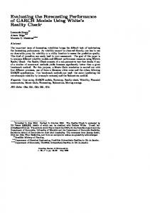
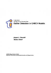
4. Data Our data set consists of 1699 daily Nord Pool closing prices for spots and futures contracts between Jan-1996 and Nov-2002. The insample period for which the estimation and the specifications tests are done covers the first 1400 observations from Jan-1996 to Aug-2001. In order to achieve some comparability with previous studies, we follow the example of Byström (2003) by estimating and performing the tests using only one futures strategy. Since the short-term future contracts are more liquid as well as more correlated with the underlying spot, we will select to use futures with three weeks left to maturity. In order to avoid inclusion of thin market and expiration effects, the futures contract is rolled over one week prior to its expiration. Table 1 reports some descriptive statistics of the price levels and returns on the spot price and the futures strategy (see Figure 1). As reflected by the high JarqueBera statistics, the returns series are characterized by strong skewness and kurtosis. Quite expectedly also the null hypothesis of no GARCH effect is readily rejected by the Ljung-Box tests on squared returns. Further, we recognize that the two series are cointegrated, which suggests that an ECM specification is appropriate for modelling. For the Johansen procedure, the trace and the maximum eigenvalue test statistics are considered: the first row gives the statistic for the null hypothesis of no cointegrating vectors r = 0 for both tests while the second row shows the values associated with the hypothesis r ≤ 1 for the trace test and r = 1 for the maximum eigenvalue test. The Johansen’s tests point out that there is a cointegrating vector at 1% significance level. Visual inspection of the sample autocorrelation functions suggests slight serial correlation (Figure 2). The Ljung-Box statistics support this finding. However, before moving on to the model selection, it is important to acknowledge the problems associated with Ljung-Box tests. As discussed by Chen (2002), it is difficult to tell whether the rejections of null hypotheses by Ljung-box Q-tests are due to GARCH or other types of nonlinearities. According to his study, the LjungBox Q-tests are not robust to tail behavior which makes it difficult to rely on them in constructing ARMA-GARCH models. This is particularly problematic for our study of electricity prices, since the data exhibits very heavy tails that can distort the asymptotic null distributions associated with the Ljung-Box tests hence reducing their power. These are issues that require careful inspection, but as of yet there are no tests for serial correlation and volatility clustering that are robust to general nonlinearity and conditional heteroskedasticity. Therefore we will leave this as an issue for further studies, but it is nevertheless important to keep in mind the fundamental frailty of these test statistics.

5. Results The estimation is done in two steps. First, we estimate the mean equation to get the residuals, and then we estimate the conditional covariance matrix parameters using maximum likelihood, treating the residuals as observable data. The block diagonality of the information matrix under this setup guarantees that consistency and efficiency are not lost. This follows the two-step approach of Pagan and Schwert (1990), Gallant, Rossi, and Tauchen (1992), and Engle and Ng (1993).


11

5.1. Error correction model. Using a sequence of LR-ratio tests for different VAR orders, it appears that a 2-lag ECM specification effectively whitens most of the serial correlation in the returns series. This seemed to be the case even though the second lag autocorrelation is negligible. The remaining 12th order autocorrelation in the futures returns series is generated by the roll over strategy used in construction of the futures price series. As the contract is rolled over every two weeks it is likely to generate high order autocorrelation. Therefore we will consider this as a technical effect rather than something we should hunt down by including higher lag orders. Otherwise the test statistics show no surprises and the null of no serial correlation in squared residuals is rejected based on Portmanteau test. The estimated model coefficients and descriptive statistics of the non-standardized residuals are presented in Table 2. The order selection matches with previous studies as Byström (2003) used a VAR(2) model for the estimation. The inclusion of an ECM term, however, deviates from the approach chosen by Byström (2003), who excluded the error correction mechanism and instead estimated the system as a plain vector autoregression. However, given the highly significant error correction term, it is justified to use the ECM model in order to avoid downward biased in hedge ratios. 5.2. Univariate diagnostics and goodness-of-fit. The standard way to model conditional variances is to use GARCH(1,1)-filter with different underlying distributions, which provides an easy way for preliminary evaluation. In Table 3. we have computed standard diagnostics for the univariate GARCH specifications obtained from CCORR. The statistics indicate that the null of no asymmetric effects in the conditional variance is rejected based on the sign and size bias tests proposed by Engle and Ng (1993). But overall the simple GARCH(1,1) specification appears to be quite good, since the rest of the statistics are insignificant and the model parameters are relatively stable. However, a word of caution is necessary. As with many tests, the power of the statistics is not very high and rejection of the null hypothesis by one or several of the tests does not give much information concerning which nonlinear GARCH model might be the appropriate alternative. The same problem concerns the direct tests against QGARCH and LSTGARCH. As a next step, we tested the goodness-of-fit of different underlying distributions for both marginal distributions and their dependence structure. The results are furnished in Table 4. The Panel A provides Kolmogorov-Smirnov tests using t-distribution, GED-distribution and normal distribution to estimate GARCH(1,1) for the spot and futures returns separately. The tests indicate that the null hypothesis of normal distribution is strongly rejected, whereas the null of Student’s t-distribution or GED-distribution appears to be a more appropriate choice as a marginal distribution. However, when we move on to test the dependence structure between the two series the findings are somewhat different. As represented in Panel B, the copula statistics proposed by Chen et al. (2004) suggest that the normal copula or normal-DCC copula, where the correlation structure is dynamic, would be more appropriate than the Student’s t-copula. This finding is quite interesting from the practitioner’s point of view, since although we would reject joint normality of returns based on Kolmogorov-Smirnov tests, the bivariate normal copula is still a reasonably good model for the dependence structure. Therefore the choice between using exclusively normal distribution or t-distribution is not clear cut in our case.

12


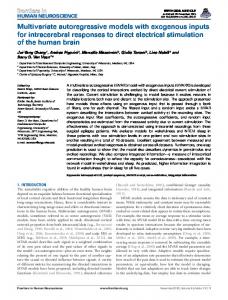
This is one of the reasons why we have estimated the range of multivariate GARCH models using both normal and Student’s t-distribution. However, the finding that a normal copula can be still a viable model for dependence structure even though the marginal distributions would be non-normal, is well documented especially in the case of bivariate models. Recently Malevergne and Sornette (2003), among others, have presented evidence that the bivariate normal copula hypothesis cannot be rejected for many pairs of equity returns, but when moving to a larger collections of financial assets Mashal and Zeevi (2002) find that a multivariate normal copula is more easily rejected in favor of a multivariate Student’s t-copula. 5.3. Comparison of MGARCH models. Having tested the univariate GARCH model, we are ready to compare the range of MGARCH models selected for the study. This section is outlined as follows. First we will shortly present the estimation results of the four models specified in the previous section. Then we will consider the summary statistics of the variance and covariance series obtained from the different models. In the first MGARCH model the spot and futures returns are modelled within the bivariate conditional correlation (CCORR) framework. The conditional variance equations are specified as GARCH(1,1) for the two series. The estimation results for the model are presented in Table 5. The left hand side of the table presents the parameters for the spot variance and on the right for the futures variance. Judging from the highly significant correlation coefficient the spot and futures returns are highly correlated. The correlation is also quite stable, since the DCC-statistics in Panel B do not seem to lend much support for a dynamic correlation coefficient. The residual statistics in the lower part of the table show that the first order GARCH model has been sufficient to remove the serial correlation from the squared residuals. However, the fact that we observe high kurtosis in standardized residuals, suggests that a different distributional hypothesis could prove useful. Alternatively it could be interesting to consider whether some other nonlinear models than GARCH would do a better job. However, we will leave this as an issue for further studies. Having changed the underlying distribution, we have estimated the diagonal TBEKK, the full T-BEKK and also Asymmetric T-BEKK to consider the potential asymmetric effects. The estimation results of these models are furnished in Table 6. The descriptive statistics below the table confirm that the assumption of GARCH disturbances removes effectively the autocorrelation in the squared residuals as in the CCORR case. The estimated variance, covariance and hedge ratio series are shown in Figures 3 to 6. As a next step we will consider the summary statistics of the variance and covariance series obtained from these models. These summary statistics, including the mean, standard deviation, minimum, and maximum, are reported in Table 7. For further intuition, we have reported the correlations between the estimates in Table 8. The findings from Tables 7 and 8 are aligned with the argument of Kroner and Ng (1998) that the multivariate GARCH models give quite different variance and covariance estimates. For futures variances the CCORR estimates are considerably more volatile than the BEKK estimates, but the situation is reversed, when we consider the covariances; the BEKK models produce a broader range of covariance estimates, as evidenced by the large maximum-minimum range. The effect of the tdistribution is pronounced as higher spot variances and lower futures variances when benchmarked against the models using normal distribution. When considering the


13

estimated hedge ratios from different models, we find that the use of t-distribution appears to lead to smaller hedge ratios and higher standard deviation than the normal distribution. Also the full BEKK models give smaller hedge ratios than the diagonal models. The correlations reported in Table 8 evidence the differences between normal and t-distribution quite expectedly, but in addition we find that the covariance estimates from the asymmetric T-BEKK and hence also the hedge ratios are negatively correlated with the rest of the models. This is a somewhat odd finding, as it is difficult to design any good explanation why this should be the case. The results from robust conditional moments tests as suggested by Kroner and Ng (1998) are displayed in Table 9. When taking a look at the broader picture, we could say that from a practitioner’s point of view the findings are quite good as only a few misspecifications are detected. Further, in terms of these tests there are no major differences between the various models as judged by the statistics computed for spot variance and covariance series. The spot variance statistics furnished in Panel A indicate some heteroskedastic asymmetry problems in CCORR, diagonal BEKK and diagonal T-BEKK as they all appear to suffer from the combination, where a negative futures shock occurs with a large spot shock. The covariance statistics in Panel B are even better, as all the other models clear out completely except CCORR, which has heteroskedastic asymmetry problem with negative spot shock combined with large futures innovation. Only futures variance seems to suffer from broader misspecifications. All of the models are misspecified with respect to negative spot returns shocks and combination of positive spot and positive futures returns shocks. CCORR has also the heteroskedastic asymmetry problem as in the case with covariances. Additionally the diagonal models and asymmetric T-BEKK suffer from combination, where positive spot return shock occurs with a negative futures shock. Overall, if we were to rank the models by these test statistics, TBEKK would be the best candidate for further modelling and CCORR the worst. The greatest problem is that all of the models are bad at capturing the asymmetric relationship between futures and shocks to the spot returns. 5.4. Evaluation of hedging performance. Additionally, following the example of Byström (2003) we have compared the hedging performance of the different models using both unconditional and conditional measures. The models selected for the outsample tests are CCORR, Diag-BEKK, Diag T-BEKK, and T-BEKK. Given that the robust conditional moments tests that were performed in the previous section indicated no substantial need for inclusion of asymmetric terms, we have decided to leave out Asym T-BEKK due to the large computational costs involved in the estimation of the model and the apparent lack of benefits over the traditional models as measured by the conditional moments tests. In the unconditional method the mean and variance of the returns of the hedged portfolios and the percentage reduction in the variance of the hedged portfolio relative to the unhedged portfolio are calculated as ru = St+1 − St rh = ru − ht (Ft+1 − Ft ) V R = 1 − σr2h /σr2u

14


where St , Ft , ru , rh , and VR denote the logarithmic spot price, logarithmic futures price, return of unhedged portfolio, return of hedged portfolio, and variance reduction, respectively. The conditional variance method proposed by Byström (2003) is based on a similar idea. However, we start by assuming that the true return and variances processes are generated by one of the GARCH models under consideration. This gives us the possibility to compare the relative performance of the data generating GARCH and the other models in minimizing the conditional variance. Hedging the spot portfolio each day and then taking the average of the conditional variance of the spot and the hedge portfolio yields us a measure for each portfolio that should be as small as possible. The test results are summarized in Table 10. Starting with the unconditional variances reported in Panel A, we find that all hedges except the naive hedge reduce the portfolio variance compared to the spot variance. Somewhat surprisingly, the best hedge in both in-sample and out-of-sample seems to be the ECM-hedge. At this point, it would appear that there is not much point in using the elaborate multivariate models as the simple ECM readily achieves equal or even better results. The findings are quite similar to those made by Byström (2003) who studied weekly portfolio returns. However, unlike Byström (2003) we do not find the naive hedge better than other hedges - on the contrary it appears to consistently increase the portfolio variances. Further we find a clear difference between the in-sample and out-of-sample performance. The models using Student’s t-distribution appear to perform better in the out-of-sample than in-sample. But once we move to inspect the reduction of the conditional instead of the unconditional variances, the obtained messages are quite different. In Panel B, the average conditional variance and the variance reductions (both in-sample and outof-sample) of the different hedges compared to the open spot position are presented for the four different choices of the underlying covariance matrix. As anticipated, we find that the ECM-hedge and naive hedge both increase the portfolio variance in the in-sample and out-of-sample comparisons as they are not able to account for the time variations. Further, it is a stylized fact that those models that are assumed to generate the underlying covariance matrix perform well. For example, when considering the variance reduction achieved by T-BEKK model and assuming that it also generates the covariance matrix, we are not surprised to find that the model also gives the best results as benchmarked against its competitors. Yet, there are some exceptions. An interesting finding is that the diagonal BEKK appears to perform well throughout the comparisons, whereas CCORR is successful only in case we assume that it is the matrix generating model. Generally also Diag T-BEKK and T-BEKK perform well, yet the Diag BEKK is even better in the outsample tests. However, none of these models was able to achieve conditional variance reductions greater than 4.97%. Overall, in the performance of these hedge ratios, the in-sample and out-ofsample comparisons tell a similar story. It is evident that the non-hedged spot position is more volatile than the hedged portfolios. Also use of an appropriate hedging model instead of a naive hedge or no hedge at all is important from variance minimizer’s perspective. This finding is consistent with Byström’s (2003) study, who finds that the inclusion of heteroskedasticity and volatility clustering in calculating the hedge ratio clearly contributes towards an optimal hedge when looking at the conditional variance. However, the selection of the model to be


15

used in daily hedging, depends on whether we want to minimize the conditional or unconditional portfolio variance. Based on these hedging performance evaluations only, it is difficult to discriminate between the different MGARCH models. Unconditional tests would recommend the use of either ECM-hedge or T-BEKK based on the out-of-sample tests, whereas the conditional tests suggest that Diagonal BEKK, Diagonal T-BEKK, and T-BEKK are almost equally good candidates for daily hedging. In the light of the robust conditional moments tests and other statistics computed in the previous section, these findings are something that could have well been expected. Given, that all of the models appeared to be relatively well specified in terms of the conditional moments tests, it would have been somewhat surprising to find major differences in the hedging performance tests.

6. Conclusions The selection of appropriate hedging models has been historically a perennial source of debates. Particularly due to asset non-storability the electricity markets, have struggled with the problem of finding a correctly specified model for dynamic hedging. Thus, in order to get a more thorough insight into the model selection, we have chosen to perform a range of tests to evaluate the most commonly applied MGARCH models - including the robust conditional moments tests along with the recently introduced copula statistics of Chen et al. (2004). The first part of the study is concerned with the goodness-of-fit tests and robust conditional moments tests, where the purpose is to examine whether the models are appropriately specified by testing them against the presence of different kinds of asymmetric effects. The second part of the study focuses more on the hedging performance of the different models based on conditional and unconditional immunized portfolio variances. The purpose is to inspect the sensitivity of hedging results to model selection. Starting with the goodness-of-fit tests for different underlying distribution candidates and copula statistics, we made a few interesting findings that could guide further studies in the area. These were issues concerned with the choice of underlying marginal distributions and their dependence structure. The problem with the traditional multivariate GARCH models that we have studied so far is that they compel us to use exclusively one distribution to model the whole covariance matrix even though a combinatorial approach could be preferable. In this study we have many times rejected the assumption of normality of the spot and futures series, yet still accepted the use of normal copula to be a more appropriate choice for the dependence structure than the Student’s t-copula. Although, also a t-copula appeared to be adequately good for modelling the dependence structure. Thus, the problem we have faced in the use of the multivariate GARCH models selected for this study, is that all of them are misspecified in some respect: when using CCORR and diagonal BEKK we have misspecified the marginal distributions by assuming them to be normal, but when using diagonal T-BEKK, T-BEKK or asymmetric T-BEKK we have problems with the dependence structure. The model that could prove more effective would be one that combines the best of the both sides: marginal Student’s t-distributions with normal copula as the dependence structure. However, having made the decision to focus on the commonly applied MGARCH models, we decided to continue with a collection of models using both gaussian and Student’s t-copulas.

16


The second step was to evaluate the models in the spirit of Kroner and Ng (1998) using the robust conditional moments tests for potential asymmetries. In general the findings were good from a practitioner’s point of view, since all of the models studied appeared to be relatively well specified. Only futures variance specifications suffered from some asymmetric effects. All of the models appeared to be misspecified with respect to negative spot return shocks and a combination of positive spot and positive futures return shocks. T-BEKK appeared to have the least number of rejections. The diagonal models suffered from the combination where positive spot return shocks occur with negative futures return shocks, and CCORR had heteroskedastic asymmetry problems also with the covariance specification. Overall the tests implied surprisingly weak evidence on unaccounted asymmetries, which suggests that although the models fail to capture some asymmetric responses to shocks the need to incorporate these effects into models is not too acute. The third step of the study was to consider the hedging performance differences by comparing the conditional and unconditional immunized portfolio variances. As Byström (2003), we find that when comparing the results from the conditional evaluation with the results from the unconditional evaluation, there are both similarities and differences. In both cases, it is quite obvious how hedging in the electricity markets can reduce the variance, but when conditional metrics are used the inclusion of the ARCH effects in calculating the optimal hedge ratio clearly suggests that GARCH models contribute towards the optimal hedge ratios. The evidence was stacked against the naive hedge strategy throughout the comparison and also the simple ECM-hedge and CCORR achieved weaker results than the Diagonal BEKK models and T-BEKK. However, the selection between MGARCH and ECM-hedges depends on whether we want to minimize the conditional or unconditional variance. If conditional variance is considered, the MGARCH approach should be preferred but if only unconditional variance is considered then the simple ECM-hedge would best out all the rest of the models. Overall, it has shown to be quite difficult to say whether any particular MGARCH model should be preferred. Rather we have been surprised by how little differences the tests have managed to reveal between the models. For a practitioner the message is positive: one just needs to choose the simplest model that is not too badly specified in terms of the conditional moments tests. In this case the choice would be between the Diagonal specifications and the full T-BEKK - each of them yielding relatively similar hedging benefits. Much research remains to be done in this area. One major issue is the problem of finding an appropriate underlying distribution. The tests performed in this study have readily indicated that neither the gaussian nor Student’s t-distribution appear to provide full fit. Rather than being a problem of a technical model specification as studied by the robust conditional moments tests, the bigger problem is in the selection of the marginal distributions and their dependence structure. Finally, given that the whole study was flooded with different specifications tests and diagnostics, it became quite clear that a perennial source of new research issues is the design and comparison of new techniques. In particular, the analysis of multivariate non-linear models has been taken up only very recently, and currently there are no generally accepted ideas on how to construct and test such models in the first place. One of the fundamental problems is the inability of traditional Ljung-Box Q tests to distinguish between serial correlations and the volatility clustering effects. As discussed by Chen (2002), the lack of robust portmanteau tests for volatility


17

clustering makes it difficult to judge whether one should use GARCH models or other nonlinear models such as conditional heteroskedastic higher-order moments. Thus, it seems that much further research is needed on issues as representation, specification, estimation, inference and forecasting for these models. BIBLIOGRAPHY Attanasio, O. (1991). Risk, time-varying second moments and market efficiency. Review of Economic Studies, 58, 479–494. Barz, G., Johnson, B. (1998). Modeling the prices of commodities that are costly to store: the case of electricity. In: Proceedings of the Chicago Risk Management Conference. Bekaert, G., Harvey, C. (1997). Emerging equity market volatility. Journal of Financial Economics, 43, 29–77. Bekaert, G., Wu, G. (2000). Asymmetric volatility and risk in equity markets. Review of Financial Studies, 13, 1–42. Benninga, S., Oosterhof, C. (2002). Hedging with forwards and puts in complete and incomplete markets. Research report, University of Groningen. Bollerslev, T. (1986). Generalized autoregressive conditional heteroskedasticity. Journal of Econometrics, 31, 307–327. Bollerslev, T. (1990). Modeling the coherence in short-run nominal exchange rates: a multivariate generalized ARCH approach. Review of Economics and Statistics, 72, 498–505. Bollerslev, T., Engle, R.F., Wooldridge, J.M. (1988). A capital asset pricing model with time-varying covariances. Journal of Econometrics, 96, 116–131. Byström, H. (2003). The hedging performance of electricity futures on the Nordic power exchange Nord Pool. Applied Economics, 35, 1–11. Chen, Y.-T. (2002). On the robustness of Ljung-Box and Mcleod-Li Q tests: a simulation study. Economics Bulletin, 3, 1–10. Chen, X., Fan, Y., Patton, A. (2004). Simple tests for models of dependence between multiple financial time series, with applications to U.S. equity returns and exchange rates. Working paper, London School of Economics. Clewlow, L., Strickland, C. (2000). Energy Derivatives: Pricing and Risk management. Lacima Publications. Davison, M., Anderson, L., Marcus, B., Anderson, K. (2002). Development of a hybrid model for electrical power spot prices. IEEE Transactions on Power Systems, 17, 257–264. Engle, R. (1982). Autoregressive conditional heteroskedasticity with estimates of the variance of U.K. inflation. Econometrica, 50, 987–1007.

18


Engle, R., Kroner, K. (1995). Multivariate simultaneous generalized ARCH. Econometric Theory, 11, 122–150. Engle, R., Ng, V. (1993). Measuring and testing the impact of news on volatility. Journal of Finance, 48, 1749–1778. Engle, R., Ng, V., Rothschild, M. (1990). Asset pricing with a factor-ARCH structure: empirical estimates for treasury bills. Journal of Econometrics, 45, 213–237. Engle, R., Sheppard, K. (2001). Theoretical and empirical properties of dynamic conditional correlation multivariate GARCH. Working paper, Department of Economics, UCSD. Gallant, R., Rossi P., Tauchen G. (1992). Stock prices and volume. Review of Financial Studies, 5, 199–242. Ghosh, A. (1993a). Cointegration and error correction models: intertemporal causality between index and futures prices. The Journal of Futures Markets, 13, 193–198. Ghosh, A. (1993b). Hedging with stock index futures: estimation and forecasting with error correction model. The Journal of Futures Markets, 13, 743–752. Hagerud, G. (1997). A new non-linear GARCH model. PhD thesis, Stockholm School of Economics. Harrison, M., Pliska, S. (1981). Martingales and stochastic integrals in the theory of continuous trading. Stochastic Processes and their applications, 11, 215–260. Harris, J., Stocker, H. (1998). Handbook of Mathematics and Computational Science, New York: Springer. Herbst, A., Kare D., Marshall, J. (1989). A time varying, convergence adjusted, minimum risk futures hedge ratio. Advances in Futures and Options Research, 6, 137–155. Hirshleifer, J. (1988). Price Theory and Applications, Prentice-Hall. Holmes, P. (1995). Ex ante hedge ratios and the hedging effectiveness of the FTSE100 stock index futures contract. Applied Economics Letters, 2, 56–59. Holmes, P. (1996). Stock index futures hedging: hedge ratio estimation, duration effects, expiration effects and hedge ratio stability. Journal of Business Finance and Accounting, 23, 63–77. Hong, Y., Li, H. (2002). Nonparametric specification testing for continuous-time models with applications to spot interest rates. Working paper, Humboldt Universitaet Berlin. Huisman, R., Mahieu, R. (2001). Regime jumps in electricity prices. ERIM Report Series, Erasmus University Rotterdam.


19

Kaminski, V. (1997). The challenge of pricing and risk managing electricity derivatives. In: P. Barber, ed., The US Power Market. Risk Publications. Koutmos, G., Tucker, M. (1996). Temporal relationships and dynamic interactions between spot and futures stock markets. The Journal of Futures Markets, 16, 55–69. Kroner, K., Sultan, J. (1993). Time-varying distributions and dynamic hedging with foreign currency futures. Journal of Financial and Quantitative Analysis, 28, 535–551. Kroner, K., Ng, V. (1998). Modeling asymmetric comovements of asset returns. Review of Financial Studies, 11, 817–844. Lien, D., Luo, X. (1994). Multi-period hedging in the presence of conditional heteroskedasticity. The Journal of Futures Markets, 14, 927–955. Lien, D. (1996). The effect of the cointegrating relationship on futures hedging: a note. The Journal of Futures Markets, 16, 773–780. Lindahl, M. (1992). Minimum variance hedge ratios for stock index futures: duration and expiration effects. The Journal of Futures Markets, 12, 33–53. Lundbergh, S., Teräsvirta, T. (1998). Evaluating GARCH models. Working papers in Economics and Finance, Stockholm School of Economics. Malevergne, Y., Sornette, D. (2003). Testing the gaussian copula hypothesis for financial assets dependencies. Quantitative Finance, 3, 231–250. Mashal, R., Zeevi, A. (2002). Beyond correlation: extreme co-movements between financial assets. Working paper, Columbia University. Musiela, M., Rutkowski, M. (1997). Martingale Methods in Financial Modeling. Springer-Verlag. Myers, R. (1991). Estimating time-varying optimal hedge ratios on futures markets. Journal of Futures Markets, 11, 39–53. Myers, R., Thompson, S. (1989). Generalized optimal hedge ratio estimation. American Journal of Agricultural Economics, 71, 858–868. Pagan, A., Schwert, G. (1990). Alternative models for conditional stock volatility. Journal of Econometrics, 45, 267–290. Park, H., Bera, A. (1987). Interest rate volatility, basis, and heteroskedasticity in hedging mortgages. The American Real Estate and Urban Economics Association, 15, 79–97. Peck, A. (1976). Futures markets, supply response and price stability. Quarterly Journal of Economics, 90, 407–423.

20


Purcell, W., Hudson, M. (1985). The economic roles and implications of trade in livestock futures. In: Peck, A. ed., Futures Markets: Regulatory Issues. American Enterprise Institute for Public Policy Research. Rossi, E., Zucca, C. (2002). Hedging interest rate risk with multivariate GARCH. Applied Financial Economics, 6, 121–148. Sim, A., Zurbruegg, R. (2001). Optimal hedge ratios and alternative hedging strategies in the presence of cointegrated time-varying risks. The European Journal of Finance, 7, 269–283. Skadberg, J., Futrell, G. (1966). An economic appraisal of futures trading in livestock. Journal of Farm Economics, 48, 1485–1489. Wooldridge, J. (1990). A unified approach to robust, regression-based specification tests. Econometric Theory, 6, 17–43. Yang, J., Awokuse, T. (2002). Asset storability and hedging effectiveness in commodity futures markets. Working paper, University of Delaware.


Table 1. Descriptive statistics. Panel A reports summary statistics and unit root tests of the logarithmic spot and futures prices for the full sample period between Jan-1996 and Nov-2002. ADF and KPSS denote the Augmented Dickey-Fuller test and Kwiatkowski-Phillips-Schmidt-Shin test, respectively. The trend is included in the tests. ADF tests the null hypothesis of a unit root, whereas KPSS tests the null of stationarity. The critical values for ADF are -4.0 and -3.5 at 1% and 5% levels. The corresponding critical values for KPSS are 0.216 and 0.146 for 1% and 5% levels. Q(k) is the Ljung-Box test for autocorrelation. 99% critical value for Jarque-Bera is 9.21. Panel B reports the Johansen cointegration test for spots and futures. For the Johansen’s trace test and the eigenvalue test, the first row tests the null of no cointegration and the second row tests the null of one cointegrating vector. The lag orders used in the unit root and cointegration tests were selected using a sequence of Lagrange ratio tests for VARs of different orders. Italic-bold denotes rejection at 1% significance level. Panel A: Descriptive statistics and unit root tests Spot Futures Price levels Returns Price levels Returns Mean 5.973 0.000 4.974 0.000 Standard deviation 0.397 0.082 0.038 0.038 Skewness -0.159 1.216 0.092 1.154 Excess kurtosis 0.153 37.176 -0.551 11.425 Jarque-Bera test 8.839 98200.630 23.884 9612.183 Q(4) − 32.456 − 7.094 Q2 (4) − 289.409 − 6.136 Q(12) − 40.328 − 54.663 Q2 (12) − 289.877 − 268.687 ADF -3.907 -48.734 -1.507 -47.975 KPSS 4.063 0.014 6.869 0.047

r=0 r=1

Panel B: Cointegration tests Eigenvalue test 113.337 3.284

Trace test 116.621 3.284

21

22

MULTIVARIATE GARCH MODELS IN NORDIC ELECTRICITY MARKETS Spot returns 0.4

0.2

0

−0.2

−0.4 1996

1997

1998

1999

2000

2001

2002

2003

2001

2002

2003

2001

2002

2003

2001

2002

2003

Futures returns 0.4 0.3 0.2 0.1 0 −0.1 −0.2 −0.3 1996

1997

1998

1999

2000

Squared spot returns 0.2

0.15

0.1

0.05

0 1996

1997

1998

1999

2000

Squared futures returns 0.12 0.1 0.08 0.06 0.04 0.02 0 1996

1997

1998

1999

2000

Figure 1. Spot and futures returns

MULTIVARIATE GARCH MODELS IN NORDIC ELECTRICITY MARKETS A.C.F. of spot returns, LBQ = 43.43 0.3 0.2 0.1 0 −0.1 −0.2 2

4

6

8

10

12

14

10

12

14

10

12

14

10

12

14

P.A.C.F. of spot returns 0.3 0.2 0.1 0 −0.1 −0.2 2

4

6

8

A.C.F. of futures returns, LBQ = 56.60 0.3 0.2 0.1 0 −0.1 −0.2 2

4

6

8 P.A.C.F. of futures returns

0.3 0.2 0.1 0 −0.1 −0.2 2

4

6

8

Figure 2. Autocorrelations

23

24


Table 2. ECM model estimates. The table reports the estimates of the ECM(2) for the mean in daily spot and futures prices (the first 1400 observations: between Jan-1996 and Aug2001). The futures strategy is based on buying contracts with three weeks left to maturity and rolling over one week prior to expiration. Q(k) denotes the Ljung-Box test for the first k lags. The model order was selected using a series of Lagrange ratio tests. Q2 (k) is the Ljung-Box test for the squared residuals. 99% critical value for Jarque-Bera normality test is 9.21. Italic-bold denotes rejection at 1% significance level.

Variable ∆ ln St−1 ∆ ln St−2 ∆ ln Ft−1 ∆ ln Ft−2 EC term Constant Mean Stand.dev Skewness Excess kurtosis Jarque-Bera test Q(4) Q2 (4) Q(12) Q2 (12)

Spot Estimates t statist. -0.052 -1.894 -0.042 -1.613 0.372 6.400 0.019 0.329 −0.021 -9.757 0.002 0.900

Futures Estimates t statist. -0.014 -1.064 -0.003 -0.227 0.029 1.023 -0.033 -1.147 -0.002 -2.196 0.000 0.285

0.000 0.082 2.313 39.115 90301.857 2.730 121.390 7.531 121.685

0.000 0.040 1.136 10.292 6465.328 4.495 5.730 57.212 213.697


Table 3. Univariate GARCH diagnostics. The table gives diagnostic tests for the univariate GARCH specifications obtained from CCORR. The ARCH and GARCH tests denote the LM-test proposed by Lundbergh and Teräsvirta (1998). The sign and size bias tests of standardized residuals are based on Engle and Ng (1993). QGARCH and LSTGARCH denote the direct tests against these alternatives as proposed by Hagerud (1997). The parameters constancy tests denote the Lundbergh and Teräsvirta (1998) tests against ANST-GARCH.

No remaining ARCH Higher order GARCH GARCH vs. QGARCH GARCH vs. LSTGARCH Intercept stability ARCH parameter stability All parameters stability Sign Bias Positive Size Bias Negative Size Bias Sign and Size Bias

Spot Futures Statistic P-value Statistic P-value 0.022 0.883 1.505 0.220 0.043 0.835 1.347 0.246 0.221 0.638 2.089 0.148 0.078 0.780 2.147 0.143 2.292 0.130 1.673 0.196 0.890 0.346 0.926 0.336 2.418 0.490 1.955 0.582 -1.775 0.038 -1.587 0.056 44.434 0.000 31.919 0.000 -2.554 0.005 -13.036 0.000 960.106 0.000 1018.965 0.000

Table 4. Goodness-of-fit tests for distributions. K-S Tdist, K-S GED-dist and K-S Normal-dist statistics represent the Kolmogorov-Smirnov tests the null that the errors are from the given distribution. The N(0,1) distributed copula statistics are based on the work of Chen et al. (2004). Panel A: Marginal distribution Spot Futures K-S T-dist 0.035 (0.059) 0.030 (0.173) K-S GED-dist 0.037 (0.047) 0.032 (0.106) K-S Normal-dist 0.118 (0.000) 0.093 (0.000) Panel B: Copulas Raw errors GARCH-filter Normal copula 0.427 (0.335) -0.716 (0.237) Student’s t-copula -1.785 (0.037) -1.218 (0.112) Normal-DCC copula 0.601 (0.274) -0.445 (0.328)

25

26


Table 5. CCORR and DCC-MGARCH test. The table presents the maximum likelihood parameter estimates for the constant correlation model. The lower part of the table gives standardized residual statistics. Log L denotes the loglikelihood value and Q2k denotes the Ljung-Box test for the remaining serial correlation in the squared residuals. 99% critical value for Ljung-Box is 16.8 and for the Lilliefors normality test 0.0276. The DCC-MGARCH test statistic is χ2 distributed with nlags+1 degrees of freedom. The pval denotes the probability that the correlation is constant.

ωii αii βii ρij LogL Mean Skewness Excess Kurtosis Lilliefors Test Q(6) Q2 (6)

Panel A: CCORR Spot Futures Estimates t statist. Estimates t statist. 0.003 15.962 0.000 5096.327 0.307 0.530 0.100 159.916 0.335 0.074 0.867 546.339 0.172 54.691 0.172 54.691 4315.76 0.019 -0.010 4.980 0.912 79.242 9.300 0.12 0.09 0.06 4.57 0.01 0.16

Panel B: Test against DCC-MGARCH Number of lags Statistic P-value 1 0.252 0.882 3 1.087 0.896 6 3.472 0.838 9 16.792 0.079 12 17.352 0.184 15 19.843 0.227


27

Table 6. BEKK models

Panel A: Parameter estimates of alternative models Diag BEKK Diag T-BEKK T-BEKK Asym T-BEKK ω11 ω21 ω22 α11 α12 α21 α22 β11 β12 β21 β22 g11 g12 g21 g22 ν LogL

0.050 (0.000) 0.030 (0.005) 0.003 (0.000) 0.003 (0.000) 0.006 (0.000) 0.005 (0.000) 0.524 (0.008) 0.636 (1.970) 0.253 (0.001) 0.188 (0.134) 0.596 (0.009) 0.717 (0.020) 0.953 (0.000) 0.973 (0.000) 3.176 (98.975) 4305.276 4911.540 Spot

Futures

0.031 (0.003) 0.029 (0.000) 0.000 (0.000) -0.001 (0.000) 0.006 (0.000) 0.007 (0.000) 0.682 (1.069) 0.640 (0.003) -0.343 (0.431) -0.599 (0.006) 0.002 (0.002) -0.021 (0.000) 0.177 (0.059) -0.141 (0.000) 0.683 (0.009) 0.683 (0.000) 0.095 (0.004) 0.080 (0.001) 0.002 (0.001) 0.012 (0.000) 0.975 (0.000) 0.965 (0.000) 0.286 (0.002) -0.286 (0.004) -0.008 (0.000) 0.170 (0.000) 12.261 (51.115) 3.168 (15.885) 4916.935 4924.494

Panel B: Diagnostics Spot Futures Spot

Futures

Spot

Futures

Q(1) 0.000 0.749 0.015 0.207 0.013 0.151 0.006 0.150 Q(2) 0.018 0.827 0.048 1.166 0.042 1.330 0.033 0.667 Q(5) 0.051 3.601 0.091 4.644 0.079 5.027 0.070 3.803 Q(10) 0.125 51.544 0.193 73.431 0.166 76.937 0.154 66.161 Q2 (1) 0.001 0.037 0.001 0.033 0.001 0.031 0.001 0.027 Q2 (2) 0.003 0.044 0.002 0.033 0.002 0.031 0.002 0.030 Q2 (5) 0.006 0.118 0.005 0.109 0.005 0.106 0.004 0.091 Q2 (10) 0.013 2.614 0.010 7.077 0.009 8.061 0.009 5.368 AIC -8596.551 -9807.079 -9809.871 -9816.987 SIC -8559.856 -9765.143 -9746.966 -9733.114 AIC = -2 logL+2K, where K is the number of estimated parameters and log L is the log-likelihood function. SIC = -2 logL + K log(T), where T = 1517 is the sample size and K is the number of estimated parameters and logL is the log-likelihood function

28


Table 7. Summary statistics of variances, covariances and hedge ratios. This table gives summary statistics for the variance, covariance and hedge ratio series estimated from the different MGARCH models discussed in the article. All models have been applied to the same dataset between Jan-1996 and Aug-2001. ε1t is the spot return innovation and ε2t is the innovation to the futures return. h11t , h22t , and h12t denote the estimated spot variance, futures variance and their covariance, respectively. Model Variable Mean SD Minimum Maximum Spot variance ε21t CCORR h11t 0.007 0.015 0.004 0.395 Diag BEKK h11t 0.007 0.014 0.004 0.354 Diag T-BEKK h11t 0.007 0.023 0.002 0.518 T-BEKK h11t 0.008 0.025 0.002 0.582 Asym T-BEKK h11t 0.008 0.025 0.002 0.505 Futures variance ε22t CCORR h22t 0.002 0.002 0.001 0.035 Diag BEKK h22t 0.002 0.001 0.001 0.010 Diag T-BEKK h22t 0.002 0.001 0.001 0.006 T-BEKK h22t 0.002 0.001 0.001 0.006 Asym T-BEKK h22t 0.002 0.001 0.001 0.008 Covariance ε12t CCORR h12t 0.001 0.000 0.000 0.006 Diag BEKK h12t 0.001 0.001 -0.005 0.010 Diag T-BEKK h12t 0.001 0.001 -0.005 0.010 T-BEKK h12t 0.001 0.001 -0.009 0.007 Asym T-BEKK h12t 0.001 0.001 -0.018 0.010 Hedge ratios ε12t /ε2t CCORR h12t /h2t 0.352 0.165 0.080 3.342 Diag BEKK h12t /h2t 0.379 0.318 -2.042 3.898 Diag T-BEKK h12t /h2t 0.315 0.314 -1.901 2.981 T-BEKK h12t /h2t 0.297 0.349 -2.330 4.267 Asym T-BEKK h12t /h2t 0.268 0.499 -10.296 3.553


CCORR

29

Diagonal BEKK

0.1

0.1

0.05

0.05

0 1996 1997 1998 1999 2000 2001 2002 Diagonal T−BEKK 0.1

0.05

0 1996 1997 1998 1999 2000 2001 2002 T−BEKK 0.1

0.05

0 1996 1997 1998 1999 2000 2001 2002 Asym T−BEKK 0.1

0 1996 1997 1998 1999 2000 2001 2002

0.05

0 1996 1997 1998 1999 2000 2001 2002

Figure 3. Spot variances

30


CCORR

Diagonal BEKK

0.015

0.015

0.01

0.01

0.005

0.005

0 1996 1997 1998 1999 2000 2001 2002 Diagonal T−BEKK 0.015

0 1996 1997 1998 1999 2000 2001 2002 T−BEKK 0.015

0.01

0.01

0.005

0.005

0 1996 1997 1998 1999 2000 2001 2002 Asym T−BEKK 0.015

0 1996 1997 1998 1999 2000 2001 2002

0.01 0.005 0 1996 1997 1998 1999 2000 2001 2002

Figure 4. Futures variances


CCORR

31

Diagonal BEKK

0.01

0.01

0.005

0.005

0

0

−0.005

−0.005

−0.01 1996 1997 1998 1999 2000 2001 2002 Diagonal T−BEKK 0.01

−0.01 1996 1997 1998 1999 2000 2001 2002 T−BEKK 0.01

0.005

0.005

0

0

−0.005

−0.005

−0.01 1996 1997 1998 1999 2000 2001 2002 Asym T−BEKK 0.01

−0.01 1996 1997 1998 1999 2000 2001 2002

0.005 0 −0.005 −0.01 1996 1997 1998 1999 2000 2001 2002

Figure 5. Covariances

32


CCORR

Diagonal BEKK

2

2

1

1

0

0

−1

−1

−2

−2

1996 1997 1998 1999 2000 2001 2002 Diagonal T−BEKK

1996 1997 1998 1999 2000 2001 2002 T−BEKK

2

2

1

1

0

0

−1

−1

−2

−2

1996 1997 1998 1999 2000 2001 2002 Asym T−BEKK

1996 1997 1998 1999 2000 2001 2002

2 1 0 −1 −2 1996 1997 1998 1999 2000 2001 2002

Figure 6. Hedge ratios


33

Table 8. Correlations. This table gives correlations between the variance, covariance and hedge ratio series estimated from the different MGARCH models discussed in the article. All models have been applied to the same dataset between Jan-1996 and Aug2001. Spot variance CCORR Diag BEKK Diag T-BEKK T-BEKK Asym T-BEKK Futures variance CCORR Diag BEKK Diag T-BEKK T-BEKK Asym T-BEKK Covariance CCORR Diag BEKK Diag T-BEKK T-BEKK Asym T-BEKK Hedge ratios CCORR Diag BEKK Diag T-BEKK T-BEKK Asym T-BEKK

CCORR Diag BEKK Diag T-BEKK 1.000 0.999 0.977 0.999 1.000 0.982 0.977 0.982 1.000 0.983 0.987 0.995 0.955 0.961 0.983 CCORR Diag BEKK Diag T-BEKK 1.000 0.586 0.538 0.586 1.000 0.968 0.537 0.968 1.000 0.527 0.955 0.998 0.527 0.949 0.978 CCORR Diag BEKK Diag T-BEKK 1.000 0.307 0.322 0.307 1.000 0.977 0.322 0.977 1.000 0.218 0.803 0.815 -0.192 -0.353 -0.321 CCORR Diag BEKK Diag T-BEKK 1.000 0.349 0.247 0.349 1.000 0.937 0.247 0.937 1.000 0.470 0.847 0.864 -0.783 -0.565 -0.552

T-BEKK 0.983 0.987 0.995 1.000 0.990 T-BEKK 0.527 0.955 0.998 1.000 0.976 T-BEKK 0.218 0.803 0.815 1.000 -0.604 T-BEKK 0.470 0.847 0.864 1.000 -0.780

Asym T-BEKK 0.955 0.961 0.983 0.990 1.000 Asym T-BEKK 0.527 0.949 0.978 0.976 1.000 Asym T-BEKK -0.192 -0.353 -0.321 -0.604 1.000 Asym T-BEKK -0.783 -0.565 -0.552 -0.780 1.000

34


Table 9. Robust Conditional Moments tests

I(ε1t−1 < 0) I(ε2t−1 < 0) I(ε1t−1 < 0; ε2t−1 I(ε1t−1 < 0; ε2t−1 I(ε1t−1 > 0; ε2t−1 I(ε1t−1 > 0; ε2t−1 ε21t−1 I(ε1t−1 < 0) ε21t−1 I(ε2t−1 < 0) ε22t−1 I(ε1t−1 < 0) ε22t−1 I(ε2t−1 < 0)



< 0) > 0) < 0) > 0)

< 0) > 0) < 0) > 0)

< 0) > 0) < 0) > 0)

CCORR 0.546 1.866 2.110 0.015 1.367 0.818 0.024 3.359 2.082 0.004 CCORR 0.104 0.210 0.009 0.168 0.286 0.027 0.007 0.272 3.362 0.195 CCORR 5.524 0.000 1.058 1.343 2.574 3.746 0.464 1.977 6.382 0.126

Panel A: Spot variance Diag BEKK Diag T-BEKK T-BEKK Asym T-BEKK 0.524 0.794 0.774 0.830 1.913 1.517 1.204 1.039 2.141 1.955 1.119 1.121 0.024 0.053 0.253 0.238 1.421 0.920 1.218 0.752 0.813 0.877 0.931 0.854 0.015 0.732 0.398 0.189 3.005 3.116 1.326 0.558 2.107 0.367 0.076 0.023 0.012 0.132 1.466 0.514 Panel B: Covariance Diag BEKK Diag T-BEKK T-BEKK Asym T-BEKK 0.771 0.002 1.026 1.081 1.132 0.305 1.088 1.219 2.266 1.102 0.837 1.244 1.116 0.319 1.060 0.288 0.784 0.001 1.011 1.281 0.022 0.000 0.112 0.992 1.534 0.705 0.002 0.865 1.437 0.323 0.095 0.172 0.617 1.504 0.120 0.423 0.826 1.189 0.846 0.402 Panel C: Futures variance Diag BEKK Diag T-BEKK T-BEKK Asym T-BEKK 5.708 6.492 6.379 6.870 0.013 0.010 0.006 0.000 1.034 1.397 1.293 1.525 1.503 1.640 2.056 1.541 3.108 4.007 2.566 5.259 3.185 2.911 3.735 2.942 0.310 0.367 0.123 0.240 1.627 1.752 1.817 2.233 1.418 1.165 1.573 3.862 0.954 0.168 0.001 0.000


Table 10. Portfolio variance tests. Panel A gives the unconditional daily portfolio return variance and percentage variance reduction in the insample and out-of-sample compared to the nonhedged spot position. The insample period covers the first 1400 observations between Jan-1996 and Aug-2001, the outsample period covers the last 299 observations between Aug-2001 and Nov2002. Panel B gives the daily portfolio return conditional variance (average value over the test period) and percentage reduction of this average conditional variance compared to the non-hedged spot position. The conditional variance tests assume that the true return and variance processes are generated by one of the GARCH models under consideration. Panel A: Unconditional daily portfolio variances (×100) Spot Naive ECM CCORR In-sample Variance 0.764 0.800 0.741 0.742 % Variance reduction -4.682 3.086 2.944 Out-of-sample Variance 0.258 0.285 0.251 0.253 % Variance reduction -10.802 2.549 1.859 Diag BEKK Diag T-BEKK T-BEKK In-sample Variance 0.755 0.759 0.757 % Variance reduction 1.227 0.775 0.969 Out-of-sample Variance 0.255 0.252 0.252 % Variance reduction 0.996 2.008 2.170 Panel B: Conditional daily portfolio variances (×100) Spot Naive ECM CCORR In-sample Cond.var, CCORR Cov. Matrix 0.688 0.765 0.833 0.668 Cond.var, Diag BEKK Cov. Matrix 0.677 0.733 0.801 0.673 Cond.var, Diag T-BEKK Cov. Matrix 0.744 0.812 0.877 0.743 Cond.var, T-BEKK Cov. Matrix 0.760 0.835 0.894 0.757 % Variance reduction, CCORR -11.180 -21.041 2.953 % Variance reduction, Diag BEKK -8.319 -18.402 0.547 % Variance reduction, Diag T-BEKK -9.163 -17.864 0.222 % Variance reduction, T-BEKK -9.926 -17.661 0.281 Out-of-sample Cond.var, CCORR Cov. Matrix 0.431 0.463 0.505 0.419 Cond.var, Diag BEKK Cov. Matrix 0.341 0.373 0.416 0.333 Cond.var, Diag T-BEKK Cov. Matrix 0.357 0.395 0.439 0.347 Cond.var, T-BEKK Cov. Matrix 0.363 0.414 0.450 0.355 % Variance reduction, CCORR -7.405 -17.216 2.798 % Variance reduction, Diag BEKK -9.367 -22.086 2.494 % Variance reduction, Diag T-BEKK -10.577 -22.982 2.828 % Variance reduction, T-BEKK -14.012 -23.854 2.265

35

36


Diag BEKK Diag T-BEKK T-BEKK In-sample Cond.var, CCORR Cov. Matrix Cond.var, Diag BEKK Cov. Matrix Cond.var, Diag T-BEKK Cov. Matrix Cond.var, T-BEKK Cov. Matrix % Variance reduction, CCORR % Variance reduction, Diag BEKK % Variance reduction, Diag T-BEKK % Variance reduction, T-BEKK Out-of-sample Cond.var, CCORR Cov. Matrix Cond.var, Diag BEKK Cov. Matrix Cond.var, Diag T-BEKK Cov. Matrix Cond.var, T-BEKK Cov. Matrix % Variance reduction, CCORR % Variance reduction, Diag BEKK % Variance reduction, Diag T-BEKK % Variance reduction, T-BEKK

0.669 0.641 0.711 0.731 2.870 5.209 4.514 3.718

0.672 0.643 0.710 0.733 2.334 4.970 4.658 3.557

0.674 0.648 0.715 0.724 2.078 4.232 3.948 4.736

0.419 0.326 0.342 0.350 2.766 4.298 4.228 3.711

0.421 0.330 0.342 0.351 2.401 3.297 4.119 3.328

0.424 0.333 0.346 0.350 0.424 2.447 2.997 3.559

EVALUATING MULTIVARIATE GARCH MODELS IN ...

EVALUATING MULTIVARIATE GARCH MODELS IN ...

Suggest Documents

Analytic Score for Multivariate GARCH Models

Multivariate GARCH models and Black-Litterman ... - CiteSeerX

Evaluating exponential GARCH models - S-WoPEc

GARCH Models in Applied

Bayesian Multivariate GARCH Models with Dynamic ... - Icmc-Usp

statistical inference for multivariate residual copula of garch models

Multivariate GARCH Models: Software Choice and ... - ICMA Centre

A Multivariate GARCH in - Clute Institute

Weighted bootstrap in GARCH models

Tree Structured GARCH Models

ASYMMETRIC GARCH MODELS

18 GARCH Models

Evaluating the Forecasting Performance of GARCH Models Using ...

Evaluating the Forecasting Performance of GARCH Models Using ...

GARCH 101: The Use of ARCH/GARCH Models in Applied ...

Block Dynamic Conditional Correlation Multivariate GARCH ... - GRETA

Sample and Implied Volatility in GARCH Models

Outlier Detection in GARCH Models - Tinbergen Institute

Model and distribution uncertainty in multivariate GARCH estimation: a ...

Evidence from a Multivariate GARCH#in#Mean VAR - canadian ...

Software implementation and testing of GARCH models

SMOOTH TRANSITION GARCH MODELS - Semantic Scholar

Flexible multivariate marginal models for analyzing multivariate ...

Multivariate autoregressive models with