We propose a new GARCH model with tree-structured multiple thresholds for ... the conditional variance and we also allow for non-Markovian models. ... goes into the dominant volatility (for real data, we usually subtract first a linear AR(1) esti-.
Tree Structured GARCH Models by ¨hlmann Francesco Audrino and Peter Bu
Research Report No. 91 March 2000
Seminar f¨ ur Statistik Eidgen¨ ossische Technische Hochschule (ETH) CH-8092 Z¨ urich Switzerland
Tree Structured GARCH Models Francesco Audrino Departement Mathematik ETH Zentrum and Peter B¨ uhlmann Seminar f¨ ur Statistik ETH Zentrum CH-8092 Z¨ urich, Switzerland March 2000 Abstract We propose a new GARCH model with tree-structured multiple thresholds for volatility estimation in financial time series. The approach relies on the idea of a binary tree where every terminal node parameterizes a (local) GARCH model for a partition cell of the predictor space. Fitting of such trees is constructed within the likelihood framework for non-Gaussian observations: it is very different from the well-known CART procedure for regression based on residual sum of squares. Our strategy includes the classical GARCH model and allows in a systematic and flexible way to increase model-complexity. We conclude with simulations and real data analysis that the new method has better predictive potential compared to other approaches. Keywords: Conditional variance; Financial time series; GARCH model; Maximum likelihood; Threshold model; Tree model.
1
Introduction
We propose a new method for estimating volatility in stationary financial time series; our real data examples are daily log-returns Xt = log(Pt /Pt−1 ), where Pt denotes the price of an asset at day t. The modeling technique is parametric and potentially high-dimensional: it adds thresholds, and thus partitions a predictor space, in the fashion of a binary tree. Although the binary tree reminds a bit to CART (Breiman et al., 1984), our approach is very different; we explain this below. And our modeling scheme is markedly different from autoregressive threshold models (SETAR) for conditional expectations, cf. Tong (1990): because we consider the conditional variance and we also allow for non-Markovian models. As a starting point, consider a nonparametric GARCH(1,1) model, Xt = σt Zt (t ∈ Z), 2 σt2 = f (Xt−1 , σt−1 ), f : R × R+ → R+ ,
(1.1)
where (Zt )t∈Z is a sequence of i.i.d. innovation variables with E[Zt ] = 0, Var(Zt ) = 1 and Zt independent from {Xs ; s < t}. The so-called volatility σt is then related as 2 σt2 = Var(Xt |Ft−1 ) = f (Xt−1 , σt−1 ),
1
where Ft−1 denotes the σ-algebra (the information) of the variables {Xs ; s ≤ t − 1}. The restric2 tion to model the squared volatility σt2 as a function of the previous values Xt−1 and σt−1 alone 2 is natural in finance. Note that it still generates a dependence of σt from all previous observa2 : this is the important mathematical tions {Xs ; s < t} due to the recursive definition with σt−1 difference between ARCH and GARCH models. Also, the assumption that E[Xt |Ft−1 ] ≡ 0 is a reasonable approximation for many financial time series: the substantial modeling effort goes into the dominant volatility (for real data, we usually subtract first a linear AR(1) estimate for the conditional mean). The simplest but often used example for (1.1) is the classical GARCH(1,1) model (Bollerslev, 1986), f (x, σ 2 ) = α0 + α1 x2 + βσ 2 , α0 , α1 , β > 0.
(1.2)
The unknown function f (·, ·) in (1.1) may be nonlinear and even not smooth; for example, with an asymmetry in financial trading around positive and negative return values leading to a discontinuous behavior for f (x, y) around x = 0. Estimation of f (·, ·) in generality is very difficult due to the non-observable volatility in the second argument. An iterative nonparametric estimation procedure has been proposed in B¨ uhlmann and McNeil (1999). It has the usual advantage about flexibility for f (·, ·) (although quite a few theoretical issues are not rigorously settled yet); the disadvantages are mainly: lack of performance at edges which include the high values of volatility being of particular interest in practice; complications when dealing with nonGaussian observations; sensitivity to choice of smoothing parameter. Our approach here is more in the spirit of a sieve approximation with parametric models for the nonparametric function f (·, ·). The approximation has the following principles: (1) It includes the classical GARCH(1,1) model as a simple special case, (2) It uses a binary tree type selection strategy to determine splits (thresholds) for building up an approximating multiple threshold GARCH model. The binary tree construction, where every terminal node represents a (local) three-dimensional GARCH model, is based on the likelihood in model (1.1). Issue (1) has an important link to practice: there is a quite strong believe that the classical GARCH(1,1) model is appropriate, despite its simplicity with three parameters. Our tree structured nested modeling strategy allows to verify such a hypothesis by using known selection techniques for nested models: as we will see, there is potential to improve upon the classical GARCH(1,1) for real data and we will quantify such gains in terms of prediction accuracy for volatility (rather than testing about structural properties of f (·, ·)). The likelihood driven tree method mentioned in issue (2) marks an essential difference to CART (Breiman et al., 1984): underlying an approximate normality assumption for observations, CART uses residual sum of squares. For financial data, the normality assumption for observations and the corresponding techniques are not appropriate at all and can result in very poor performance. Our approach resembles more the general tree fitting with the deviance criterion used by Clark and Pregibon (1993). Another difference to CART (or more general versions driven by deviance) is that our tree structured scheme employs a three-dimensional (local) GARCH model for every terminal node in the binary tree; CART uses only one location parameter per node. Finally, our tree GARCH is for modeling the function f (·, ·) in (1.1) and hence for the infinite past in terms of the observations; whereas CART (or versions thereof) in autoregressive modeling deals with a p-dimensional predictor space (p < ∞) from finitely many lagged observations.
2
Extending the GARCH(1,1) model in (1.2) in the direction of adding potentially high parametric complexity hasn’t been considered yet. Other versions of GARCH(1,1) with three or four parameters and a GARCH model with one or two thresholds at fixed locations (Rabemananjara and Zakoian, 1993) exist already. But there seems to be no systematic flexible route how to build up a class of models from the classical GARCH(1,1) in (1.2) to (a potentially high dimensional approximation of) the general model in (1.1). The paper here deals mainly with this latter task: we describe how this can be done and we demonstrate its power and use on simulated and real data.
2
Tree structured GARCH estimation
We describe here our methodology for approximating f (·, ·) in (1.1) by a piecewise linear function (a threshold model). The novel part thereby is the estimation of thresholds in R × R+ , where piecewise approximation functions begin and end. Our algorithm below is always based on the likelihood in the working model Xt = φXt−1 + σt (θ)Zt (t ∈ Z),
(2.1)
with σt (θ)Zt as in model (1.1), but the functional form f (·, ·) now parameterized by a threshold function fθ (·, ·) which changes in the fitting procedure. We also add here a linear autoregressive term for estimating a conditional mean (being of minor importance for many financial time series). The negative log-likelihood is then −`(φ, θ; X2n )
=−
n X
log
�
Xt σt−1 (θ)fZ (
t=2
� − φXt−1 ) , σt (θ)
2 σt2 (θ) = fθ (Xt−1 , σt−1 (θ)),
(2.2)
where fZ (·) denotes the density of the innovation Zt . The log-likelihood is always considered conditional on X1 and some reasonable starting value σ1 (θ), e.g. σ12 (θ) = Var(X1 ). The function fθ (·, ·) is parameterized as binary tree structured GARCH(1,1). It involves a partition P = {R1 , . . . Rk }, ∪kj=1 Rj = R × R+ , Ri ∩ Rj = ∅ (i 6= j) for the predictor space. Then, for every partition cell Rj , we employ a GARCH(1,1) model: the parametric form of the function then depends on P, fθ (x, σ 2 ) = fθP (x, σ 2 ) =
k X j=1
� 2 α0,j + α1,j x2 + βj σt−1 I[(x,σ2 )∈Rj ] ,
(2.3)
where θ denotes the parameter set {α0,j , α1,j , βj ; j = 1, . . . , k}. For k = 1, we have the classical GARCH(1,1) model from (1.2). The partition P = {R1 , . . . , Rk } is constructed as a binary tree (every terminal node representing a partition cell Rj ) as follows. A first threshold d1 ∈ R or R+ together with a component index ι1 ∈ {1, 2} partitions R × R+ = Rlef t ∪ Rright , where Rlef t = {(x, σ 2 ) ∈ R × R+ ; (x, σ 2 )ι1 ≤ d1 } and Rright analogously but with the relation ‘>’ instead. Then, one of the partition cells Rlef t or Rright is again partitioned with a threshold 3
d2 and a component index ι2 in the same fashion. We iterate this procedure: for the mth iteration step, we specify a pair (dm , ιm ) and an existing partition cell for further refining by splitting it into two cells. The refinement of an existing partition is here always constructed according to the following general rule: P (old) = ∪j Rj an existing partition → pick an element Rj ∗ ∈ P (old) → split Rj ∗ = Rj ∗ ,lef t ∪ Rj ∗ ,right described by (d, ι) ∈ R × {1, 2} → P (new) = ∪j6=j ∗ Rj ∪ (Rj ∗ ,lef t ∪ Rj ∗ ,right ),
(2.4)
with (d, ι) describing a threshold and component index, Rj ∗ ,lef t = {(x, σ 2 ) ∈ Rj ∗ ⊂ R × R+ ; (x, σ 2 )ι ≤ d} and analogously for Rj ∗ ,right with the relation ‘>’. The procedure then produces a partition P = {R1 , . . . , Rk } which can be represented as a binary tree: every terminal node in the tree represents a partition cell Rj . This is conceptually as in CART (Breiman et al., 1984). But the data-driven construction of a tree or partition, including the splitting operations in (2.4), and estimation of parameters are very different.
2.1
Forward entering of thresholds: growing the binary tree
The available univariate data is X1 , . . . , Xn . The algorithm below constructs a binary tree, corresponding to a partition of R × R+ , by optimizing reduction of a reduced negative loglikelihood. Thereby, binary trees are equipped with 3 parameters per terminal node for different GARCH(1,1) models for different partition cell. Step 1. Compute the negative log-likelihood from (2.2) without partitioning (i.e. in the (0) partition Popt = R × R+ ) with P
(0)
opt fθ(0) (x, σ 2 ) = α0 + α1 x2 + βσ 2 , θ(0) = (α0 , α1 , β),
and derive from it the maximum likelihood estimates φˆ(0) , θˆ(0) using a quasi-Newton method, cf. Nocedal and Wright (1999). Set m = 0. (m) Step 2. Increment m by one. Search for the best refined partition Popt by binary splitting of a cell from P (m−1) as described in (2.4). The details are as follows: (m−1) (I) Given Popt = {R1 , . . . , Rm }, consider a new partition P (m) , where one partition cell Rj ∗ ∈ P (m−1) is split into Rj ∗ = Rj ∗ ,lef t ∪ Rj ∗ ,right . The function associated with P (m) is (m)
P 2 f(θ = (m−1)\∗ ,θ ∗ ) (x, σ )
X
(α0,j + α1,j x2 + βj σ 2 )I[(x,σ2 )∈Rj ]
j6=j ∗
+
X
(α0,i + α1,i x2 + βi σ 2 )I[(x,σ2 )∈Ri ] ,
(2.5)
∗ ∗ i∈{jlef t ,jright }
where θ(m−1)\∗ = {α0,j , α1,j , βj ; j = 1, . . . , m, j 6= j ∗ } ∗ ∗ θ∗ = {α0,i , α1,i , βi ; i ∈ {jlef t , jright }}.
(II) Compute the minimal negative reduced log-likelihood in the refined partition P (m) , � � P (m) ˆ(0) ˆ(m−1)\∗ ∗ n min −` ( φ , ( θ , θ ); X ) , 2 ∗ θ
4
(2.6)
(m)
by numerical minimization over θ∗ using a quasi-Newton method. Here, −`P is as in (2.2) (m) with the function f P (·, ·) from (2.5). For this numerical minimization over θ∗ , use as starting values the components of θˆ(m−1) for cell Rj ∗ for both (θ1∗ , θ2∗ , θ3∗ ) and (θ4∗ , θ5∗ , θ6∗ ) (the parameters for the refined partition cells Rj ∗ ,lef t , Rj ∗ ,right ). (III) Optimize (2.6) by varying P (m) in (I) and recomputing (II). Denote the optimal refined (m) partition by Popt . (m)
Step 3. Compute the maximum likelihood in partition Popt . Minimize with a quasi-Newton (m) method the negative log-likelihood in (2.2) with f Popt (·, ·) from (2.5) to obtain (φˆ(m) , θˆ(m) ). Thereby, use the starting values φˆ(m−1) , θˆ(m−1)\∗ and θˆ∗ being the minimizer for (2.6) which is computed in Step 2. (M ) Step 4. Repeat Steps 2 and 3 until m = M . This yields a partition Popt corresponding to a large binary tree equipped with parameter estimates (φˆ(M ) , θˆ(M ) ). Remark 2.1. The value M , corresponding to M + 1 partition cells or terminal nodes in the binary tree, is pre-specified in advance such that the binary tree is sufficiently large. With financial return data, choosing M around 6 is often sufficient. Remark 2.2. The search for the splitting value in Step 3 is done on a grid: we propose grid-points being empirical α-quantiles of the data with α = i/mesh, i = 1, . . . , mesh − 1. We typically choose mesh = 8 or 16. Remark 2.3. The reduced log-likelihood in (2.6) yields a substantial computational short-cut compared to a full likelihood approach. For every given partition P (m) , the numerical nonlinear minimization in (2.6) involves only the 6-dimensional parameter θ∗ . Since our algorithm searches over many candidate partitions P (m) in every iteration step m, a relatively fast nonlinear minimization is important. Finding the best split is thus determined by maximal reduction of the negative reduced log-likelihood. Remark 2.4. The parameter estimates in Step 3 are computed from the full likelihood. For (φˆ(m) , θˆ(m) ) we take advantage of the fact that the starting values specified in Step 3 are very reasonable for obtaining a reliable and fast maximum likelihood estimate in a possibly high-dimensional parameter space.
2.2
Pruning the tree (M )
The binary tree, or the partition Popt , constructed in section 2.1 is too large, or too fine, respectively. We thus prune back: since M around 6 seems large enough for very many financial time series, searching for the best subtree is computationally feasible. Denote by τ the set of (M ) all binary subtrees from Popt : its elements are denoted as Pi . Thus, every Pi corresponds to a partition of R × R+ which can be represented as a binary tree. Note that τ is generally larger (0) (1) (M ) than the set {Popt , Popt , . . . , Popt }. For every Pi , we compute the maximum likelihood estimates φˆPi , θˆPi with a quasi-Newton method, according to (2.2) with f Pi (·, ·) of the form (2.3). Note that reasonable starting values are again at hand by going backwards from φˆ(M ) , θˆ(M ) in a stage-wise manner. We then consider the penalized negative log-likelihood −2`(φˆPi , θˆPi ; X2n ) + 2(dim(θˆPi ) + 1)
(2.7)
as a measure for predictive potential, namely the AIC statistic. The additional contribution 1 in the penalty term arises whenever the conditional expectation parameter φ in (2.1) is estimated. 5
ˆ minimizing (2.7). The final tree structured GARCH Choose the binary tree, or the partition P, ˆ ˆ P model is thus given by (2.1) with φˆ , and f P (·, ·) as in (2.3) based on partition Pˆ and parameter ˆ estimates θˆP . Remark 2.5. The AIC-statistic in (2.7) can be replaced by any other sensible model selection criterion. We have experimented with two other versions but found that overall performance with AIC is very satisfactory.
3
Numerical results
In this section, we consider the performance of tree structured GARCH models for simulated and real data. We compare some of the results with the GARCH(1,1) model in (1.2) and a nonparametric generalized additive model for log-transformed squared data which is described in the Appendix. We always report here with the use of M = 5 in Step 4 from section 2.1 and with grid search as described in Remark 2.2 having mesh = 8 (except in Table 3.2 with mesh = 16 in addition): these specifications already lead to good tree structured model fits, despite their somewhat simple nature. For numerical optimization, we use the quasi-Newton method from the function ‘nlmin’ implemented in S-Plus.
3.1
Simulations
The model that we use for the simulations is as in (2.1) with φ = 0 and α0,1 + α1,1 x2 + β1 σ 2 , if x ≤ d1 , 2 α0,2 + α1,2 x2 + β2 σ 2 , if x > d1 and σ 2 ≤ d2 , f (x, σ ) = α0,3 + α1,3 x2 + β3 σ 2 , if x > d1 and σ 2 > d2 ,
(3.1)
with the following parameters and thresholds d1 and d2 , α0,1 = 0.1, α0,2 = 0.2, α0,3 = 0.8, α1,1 = 0.5, α1,2 = 0.2, α1,3 = 0, β1 = 0, β2 = 0.75, β3 = 0.5 and d1 = 0, d2 = 0.5 . The parameters {α0,i , α1,i and βi } are chosen to mimic time series of real log-returns. Also, the first threshold d1 = 0 splitting the x-coordinate of the function f (·, ·) is natural in finance, saying that volatility behaves differently when the first lagged observation (log-return) is positive or negative. The p innovation distribution is chosen as standard normal Zt ∼ N (0, 1) or as scaled t6 so that 6/4Zt ∼ t6 has again variance one. We always take sample size n = 1000: for real daily data, this would correspond to about four years which is a reasonable window in which stationarity is expected to hold approximately. Estimation is here always based using the knowledge that µt = E[Xt |Ft−1 ] ≡ 0, i.e. φ = 0 in 2.1. Figures 3.1-2 display some results from the tree structured GARCH model, in comparison with the classical GARCH(1,1) in (1.2) and the GAM model described in the Appendix. FIGURE 3.1 ABOUT HERE. From Figure 3.1 we see the following for this particular case. The tree structured GARCH model with N (0, 1) innovations overestimates the number of thresholds: the first two thresholds are approximately correct. An improvement is given by the tree structured GARCH with scaled tν -distributed innovations: the thresholds and also the estimated degrees of freedom νˆ = 5.12 for the innovations are very satisfactory. The classical GARCH(1,1) with scaled tν -distributed 6
innovations yields νˆ = 4.37 and of course, it doesn’t exhibit any ‘breakpoints’ in the volatility surface. There is no surprise that the tree structured GARCH with scaled tν -distributed innovations is best, since the true model is of this form. However, the tree GARCH estimate with N (0, 1) misspecified innovations is as a quasi-maximum-likelihood fit still reasonably good. FIGURE 3.2 ABOUT HERE Figure 3.2 exploits a desirable important feature: the tree structured GARCH with scaled tν distributed innovations performs very well in regions of high conditional variance. This is not the case with classical GARCH(1,1); and the GAM fit described in the Appendix is very poor, particularly in regions of high volatility. Note the different scales for the various procedures in Figure 3.2. For quantifying the goodness of fit, we consider various statistics: Li =
n X t=1
| σt2 − σ bt2 |i , i = 1, 2,
the AIC statistic from (2.7), n X OS-Li = | σt2 − σ bt2 (Y1t−1 ) |i , i = 1, 2, Y1n a new test set t=1
where in OS-L (out-sample loss), σ bt2 (Y1t−1 ) is using the estimated model from the data X1n and evaluates it on new test data Y1t−1 being another independent realization of the data-generating process. Both, the out-sample OS-L- and AIC-statistic are measures for predictive performance; whereas the L-norms are in-sample quantities. We can’t calculate the L-norms and the OS-Lstatistics for real data examples, but they are important measures for our simulations. Detailed results are reported in Table 3.1 where we refer to data 1, data 2 and data 3 as three independent realizations from the model (2.1) with (3.1) as described p above having N (0, 1) innovations; and data 4 denotes a realization but with scaled innovations 6/4Zt ∼ t6 . Table 3.1 ABOUT HERE. We view OS-L2 as the most relevant statistic for simulations. It gives more weight to large deviations than the OS-L1 criterion, which is often appropriate when studying the estimate in regions of high volatility. The tree structured GARCH procedure consistently outperforms the classical GARCH(1,1) and the nonparametric GAM estimate (for the latter, also the out-sample performance OS-L is very bad and we don’t report it explicitly). The classical GARCH(1,1) can exhibit huge variation in out-sample accuracy OS-L, for example a poor performance in data 2. This might be due to a very flat negative log-likelihood at the observed data: see Zumbach (1999) who also proposes a remedy. Interestingly, the tree structured GARCH model exhibits here much more stability.
3.2
Two real data examples
We consider two financial instruments with 1000 daily negative log-returns Xt = −100 log(Pt /Pt−1 ) (in percentages): from the German DAX index between January 18, 1994 and November 17, 1997; and from the BMW stock price between September 23, 1992 and July 23, 1996. We consider the the tree structured GARCH model, again in comparison with the GARCH(1,1) from (1.2) (both with an additional model term φXt−1 from (2.1) for E[Xt |Ft−1 ]), and with the GAM model described in the Appendix. FIGURE 3.3 ABOUT HERE. 7
Figure 3.3 shows the result for the DAX index from a tree GARCH fit with N (0, 1)-distributed innovations. Three thresholds are fitted in the volatility surface. Graphical diagnostics for the residuals is satisfactory: with a tendency for heavier tails than standard normal. For these real-data examples, we measure goodness of fit with the AIC statistic from (2.7) and the in-sample L2 -loss, IS-L2 =
n � X t=1
σ bt2 − (Xt − µ bt )2
�2
,
ˆ t−1 . with µ ˆt = φX TABLE 3.2 ABOUT HERE. The tree structured model improves upon the classical GARCH(1,1) (both with N (0, 1)-distributed innovations) in the two real-data examples: it is more prominent for the index than for the individual stock price. This is consistent with a common belief that classical GARCH(1,1) is better for individual prices than indices.
3.3
Summarizing numerical results
The tree structured GARCH model consistently outperforms the GARCH(1,1) model in (1.2) and the nonparametric GAM model described in the Appendix: this better performance is with respect to many goodness of fit and graphical criteria. More specifically: (1) the tree structured GARCH is much better in the interesting regions where the true volatility is high, see Figure 3.2. (2) with the tree structured GARCH, the AIC statistic is consistently lower than for classical GARCH(1,1), see Tables 3.1 and 3.2. The gain in terms of out-sample performance OS-L in simulated examples is even more substantial. (3) the tree structured fitting procedure might be slightly improved by assuming scaled tν distributed innovations Zt for the likelihood in (2.2); provided that the underlying innovations are heavier tailed, which is weakly evident in Figure 3.3 for real data. See also Table 3.1. (4) the AIC-statistic is an indicator for ranking out-sample performance with the OS-Lstatistic, see Table 3.1; and pruning with AIC in (2.7) works well. (5) the nonparametric GAM model described in the Appendix is extremely poor in regions of high volatility (this problem doesn’t disappear when trying other smoothing parameters), see Figure 3.2. Issues (1), (2) and (5) indicate a strong advantage of parametric, likelihood based methods over nonparametric least squares smoothing techniques such as the GAM specification used here or multiplicative nonparametric ARCH models in Hafner (1998) or Yang et al. (1999). As pointed out in (3), the likelihood approach can be easily modified to heavier tailed innovations inducing then even more heavy tails for the observations in the model. If performance is judged with a criterion putting emphasis on accurate prediction in high volatility regions, our tree based GARCH model is clearly best among all alternative methods considered here.
8
3.4
How appropriate is GARCH(1,1) for daily returns?
The GARCH(1,1) model in (1.2) is very popular for analyzing daily log-returns of financial assets: it is often argued that it performs well despite that it has only three parameters describing a very low-dimensional model for sample size in the range of 1000. We quantify here the possible gains by using the flexible tree structured GARCH model. In virtually all examples of daily logreturn stock data, the new tree GARCH procedure improves upon the classical GARCH(1,1): the difference in performance has often quantitative magnitude as reported in sections 3.1- 3.3, with a remarkable gain for regions of high volatility. With real data, the first split has always been found in the x-axis around zero: this is compatible with the interpretation that there is an asymmetric behavior depending on the sign of the previous log-return value.
4
Concluding remarks
We have presented a tree structured GARCH model which is more flexible and accurate for prediction of volatility in financial time series than classical GARCH(1,1). The modeling strategy includes the classical GARCH(1,1) as a special case (no thresholds) and allows to increase complexity in a systematic way. Also, the new method compares very favorably with a nonparametric technique based on additive models: especially in the interesting regions where the true volatility is moderate or large. Our univariate tree structured GARCH procedure has a straightforward application in multivariate models where the conditional variance of an individual series is modeled as a function of the individual lagged values and individual lagged volatility. The multivariate cross-dependence is then modeled with cross-dependent innovations. For example, individual tree GARCH models for volatilities lead to an attractive version of the multivariate, constant conditional correlation model (Bollerslev, 1990). Another straightforward extension of our methodology is tree structured GARCH(p, q) modeling with p > 1 and/or q > 1. As already mentioned in section 1, this may be of minor importance since the general model in (1.1) is in vogue and believed to capture the most important aspects of the underlying mechanism. Rigorous statistical inference is difficult due to the nature of non-continuity with thresholds or trees. For example, if the underlying conditional variance function f (·, ·) in (2.1) is sufficiently smooth but our threshold model is fitted as an approximation, we conjecture that the (first) fitted threshold estimate has convergence rate n−1/3 with non-normal limiting distribution: this may be shown using the empirical process results from Kim and Pollard (1990). If the aim is primarily to construct better volatility forecasts, which in turn can be used for dynamic risk management (cf. McNeil and Frey, 2000), we choose the route to select a model in terms of an information/complexity criterion rather than the somewhat inappropriate structural tool of testing. As a simple solution, we use the AIC criterion: we believe and have demonstrated on numerical examples, that it can be used as a reasonable guideline.
References [1] Bollerslev, T. (1986). Generalized autoregressive conditional heteroskedasticity. J. of Econometrics 31, 307–327. [2] Bollerslev, T. (1990). Modelling the coherence in short-run nominal exchange rates: a multivariate generalized ARCH model. The Review of Economics and Statistics 72, 498– 505. 9
[3] Breiman, L., Friedman, J.H., Olshen, R.A. & Stone, C.J. (1984). Classification and Regression Trees. Wadsworth, Belmont (CA). [4] B¨ uhlmann, P. and McNeil, A.J. (1999). Nonparametric GARCH models. Preprint, ETH Z¨ urich. [5] Clark, L.A. and Pregibon, D. (1993). Tree-based models. In Statistical Models in S, pp.377– 419, auths. J.M. Chambers and T.J. Hastie. Chapman & Hall, London. [6] Hafner, C.M. (1998). Estimating high-frequency foreign exchange rate volatility with nonparametric ARCH models. J. of Statistical Planning and Inference 68, 247–269. [7] Hastie, T.J. and Tibshirani, R.J. (1990). Generalized Additive Models. Chapman & Hall, London. [8] Kim, J. and Pollard, D. (1990). Cube root asymptotics. Annals of Statistics 18, 191–219. [9] McNeil, A.J. and Frey, R. (2000). Estimation of tail-related risk measures for heteroscedastic financial time series: an extreme value approach. To appear in J. of Empirical Finance. [10] Nocedal, J. and Wright, S.J. (1999). Numerical Optimization. Springer, New York. [11] Rabemananjara, R. and Zakoian, J.M. (1993). Threshold ARCH models and asymmetries in volatility. J. of Applied Econometrics 8, 31–49. [12] Tong, H. (1990). Non-linear Time Series. A Dynamical System Approach. Oxford University Press. [13] Yang, L., H¨ardle, W. and Nielson, J.P. (1999). Nonparametric autoregression with multiplicative volatility and additive mean. J. of Time Series Analysis 20, 579–604. [14] Zumbach, G. (1999). The pitfalls in fitting GARCH(1,1) processes. Preprint. Olsen & Associates, Z¨ urich.
Appendix Estimation with log-transform and generalized additive model (GAM). A nonparametric estimate for σt2 can be derived as follows. 1. Estimate the conditional mean µt = E[Xt |Ft−1 ] by a GAM model, µ ˆt = gˆ1 (Xt−1 ) + gˆ2 (Xt−2 ), t = 3, . . . , n, with nonparametric estimates gˆi (·) obtained from a least squares backfitting algorithm, cf. Hastie and Tibshirani (1990). 2. Compute Yt = log((Xt − µ ˆt )2 ), t = 3, . . . , n. 3. In model (2.1), but with more general additive µt instead of φXt−1 , we have Yt ≈ β +log(σt2 )+ (log(Zt2 ) − β) with β = E[log(Zt2 )]. Denote by γt = β + log(σt2 ). Fit a GAM model with the transformed data Y3n , ˆ 1 (Xt−1 ) + h ˆ 2 (Xt−2 ), t = 3, . . . , n, γˆt = h ˆ i (·) obtained from a least squares backfitting algorithm with with nonparametric estimates h response variables Yt , cf. Hastie and Tibshirani (1990). 10
4. Back-transform δt = exp(ˆ γt ) ≈ exp(β)σt2 = 1c σt2 and build Rt2 = (Xt − µ ˆt )2 /δt ≈ c Zt2 . Thus, set cˆ = (n)−1
n X
Rt2 .
t=1
5. Then, set σ ˆt2 = cˆδt . 6. Iterate steps 1.-5. Thereby use weighted estimation in step 1. with weights wt = σˆ1t , where σ ˆt2 is the estimate from the previous iteration step. Stop iterating by checking convergence of σ ˆt2 and µ ˆt . A related technique is given in Yang et al. (1999): they don’t use the log-transform but work with the squared observations and dependent, uncorrelated innovations (even when not estimated).
11
f(x,sigma) 0 2 4 6 8 10
f(x,sigma) 0 2 4 6 8 10
2 1 sig .5 ma 1
2.5
0.5
-3
-2
-1
0
1
2
x
2 1 sig .5 ma 1
0.5
-3
-2
-1
0
1
2
x
f(x,sigma) 0 2 4 6 8 10
f(x,sigma) 0 2 4 6 8 10
2.5
2.5
2 1 sig .5 ma 1
0.5
-3
-2
-1
0
1
2.5
2
x
2 1 sig .5 ma 1
0.5
-3
-2
-1
0
1
x
Figure 3.1: Top left: true conditional variance f (x, σ) given by (3.1), plotted against x and σ. This is used in model (2.1) with scaled t6 -distributed innovations to simulate data (data 4 from Table 3.1) which is at the basis of the other pictures. Top right: estimated conditional variance from classical GARCH(1,1) model with scaled tν -distributed innovations (ν unknown). Bottom left: estimated conditional variance from tree GARCH model with standard normal innovations. Bottom right: estimated conditional variance from tree GARCH model with scaled tν -distributed innovations (ν unknown).
12
2
true conditional variance
tree model •
0
0.5 0.0 -0.5
1
2
3
residuals
4
1.0
• •• • ••
0
200
400
600
800
1000
••
• • • • •• •• • • • • • •••• • • ••• • •• •• • ••••••••••••••••••• •• •••• • ••••••••••••• • ••••••••••••••••••••••••••••••••••••••••••••• ••••••••••••••••••• • •••••••••• • • • • • • • • • • •• ••• •••••••••••• •• • •• • •••• • ••••• • •• • • • 0
1
2
•••
•
3
•
4
conditional variance
GARCH(1,1) •
•
•
•
6
3
•
GAM
0
1
2
•
3
4 2
• •
0
•••• • • •••• • • •• • • •••••••• •• •••••••••••• ••••••• • • • •• • •• • • •• • ••••••••••••••• ••••••••••••••••••••••••••••••••••••••••••••••••••• •••••••••••••• • • • • •• • • • • ••• •••••••••••••• • •• •••••• • •••••••••••••••••••••• • • • • •• • • •••• •••••
••
• residuals
1 0 -1
residuals
2
• •• •
•
• 4
• • •• • • •• •• • •• •••••••••••••••••••••••••••••••••••••••••••••••••••••••••••••••••••••• •• •• • • •• ••••••••••••••••••••••••••••••• •• •• •••• •••••••••••• • • • •• •••••••• • 0
conditional variance
1
2
• •
• •
•• ••• 3
4
conditional variance
Figure 3.2: Top left: simulated volatility function from model (2.1) with (3.1) and scaled t6 -distributed
innovations (data 4 from Table 3.1). Top right: residuals Zˆt from tree GARCH with scaled tν -distributed innovations (ν unknown) against true conditional variance σt2 . Bottom left: residuals Zˆt from classical GARCH(1,1) with scaled tν -distributed innovations (ν unknown) against true conditional variance σt2 . Bottom right: residuals Zˆt from GAM model (as described in the Appendix) against true conditional variance σt2 .
13
•
f(x,sigma) 05101520253035
4
• •
• • • • • • • • • • •• • • ••••• • • ••• •• •• ••• • •• •• • •• • ••• • • • • •• • • • • •••••••••••••••••••••••••••• ••••••••••••• ••••• • •••••••••••• •• ••• ••••••••••••••••••••••••••••••••••••••••••• • • • • •• • • •• • • • • • •• • •• •••••••••••••••••••••••••••••••••••••••••••••••••••••••••••••••••••••••••••••••••••••••••••••••••••••••••••••••••••••••••••••••••••••••••••••••••••••••••••••••••••••••••••••••••••••••• ••• ••••••••••••••••••••••••••••••••••••• •• ••••• ••••••••••••• •••••••••••••••••••••••••••••••••••• •• • •• •••••••••••••••••••••••••••••••••••• •• ••••••••••••••••••••••••••••••••••••••••••••••• ••••••••••••••••••••••••••••••••••••••••••••••••••••••••••• •• ••••• • • ••• • • • • ••• •• • ••• • • • • • • ••••• ••••• ••••••• •••• •••• •• ••• • • • •••• •••••••• ••• •••• ••• •• • •• • •
3 sig
ma 2
1
2 -2
4
0
residuals
• ••
6 8 4 0 2 2 x -4 -6
0
200
•
•
•
400
600
800
1000
Index
ACF 0.0 0.2 0.4 0.6 0.8 1.0
Series : abs(residuals)
2 0 -2
residuals
4
• •
• • 0
5
10
15 Lag
20
25
30
•• ••••••• • ••• • • • • ••••••• ••••••• • • • • • • ••••••• •••••••••••• • • • • • • • • • ••••••• •••••••• • • • • • • • • • ••••• ••••••••••• •••••••• -2
0
2
Quantiles of Standard Normal
Figure 3.3: Results for negative log-returns of the DAX index using tree structured GARCH with N (0, 1)-distributed innovations. Top left: estimated function f (x, σ) for the conditional variance, plotted against x and σ. Top right: residuals Zˆt = (Xt − µ bt )/b σt from the tree GARCH model against time. Bottom left and right: autocorrelation function of the absolute residuals |Zˆt | and normal-plot for the residuals Zˆt , respectively.
14
Tree structured GARCH Thresholds data 1
data 2
data 3 average
data 4
db1 db2 db3 db1 db2 db3 db1 db2 db3
= -0.044736 = 0.773178 = 0.556751 = -0.016448 = 0.468750 = 0.724830 = -0.008402 = 0.188899 = 0.981620
db1 db2 db3 db1 db2
= -0.008463 = 0.385467 = 0.313737 = -0.008463 = 0.406501
in in in in in in in in in
x σ2 σ2 x σ2 x x x σ2
–
in in in in in
x σ2 x x σ2
AIC
L1
L2
OS-L1
OS-L2
1842.201
102.8911
43.47956
0.044393
0.061369
1862.673
74.45144
25.22954
0.028189
0.043028
1885.969
101.6080
47.08707
0.032485
0.031135
1863.614
92.98351
38.59872
0.035022
0.045177
1743.976
114.0162
40.50913
0.056668
0.032445
1709.942
99.52060
50.98907
0.092520
0.020926
GARCH(1,1)
GAM
AIC
L1
L2
OS-L1
OS-L2
L1
L2
data 1
2009.407
225.6830
116.2419
0.150125
0.175476
210.2130
347.0649
data 2
2078.053
261.5570
159.4396
0.476803
0.590879
235.0034
357.5037
data 3
2073.761
284.3699
227.1664
0.140545
0.181043
294.8932
443.7396
average
2053.7403
257.2033
167.6160
0.255824
0.315799
246.7032
382.7694
1897.215
257.8995
154.1101
0.263674
0.111068
211.4139
253.5949
1818.409
265.6812
165.3186
0.324841
0.119131
data 4
Table 3.1: Estimated thresholds dˆi and goodness of fit measures for four independent simulations of model (2.1) with (3.1): with standard normal innovations (data 1, data 2, data 3) and scaled t6 innovations (data 4). The likelihood for estimation is based on standard normal innovations (data 1, data 2, data 3); for data 4, we use standard normal innovation likelihood (upper part) and scaled tν innovation likelihood with ν unknown (lower part).
15
Tree structured GARCH Thresholds
DAX
BMW
db1 = -0.354193 in db2 = 1.235410 in db3 = 1.657356 in db1 = -0.354193 in db2 = -0.889087 in db3 = 1.657356 in db4 = -0.508199 in
x σ2 σ2 x x σ2 x
db1 = -0.321663 in x db2 = 1.110003 in σ 2
GARCH(1,1)
AIC
IS-L2
2776.238
8555.143
2764.430
8507.640
3155.012
12059.22
AIC
IS-L2
2785.297
9309.807
3165.068
12063.92
Table 3.2: Estimated thresholds dˆi , the AIC-statistic and the in-sample L2 -loss IS-L2 for negative log-returns of the DAX index and the BMW stock price. The tree GARCH model (with N (0, 1)distributed innovations) is fitted with mesh = 8 (DAX, upper part; BMW) and mesh = 16 (DAX, lower part).
16