Department of Computer Science, University of Houston, Houston, TX 77204 ... the Center for Research on Parallel Computation, a National ... energy function of the atom positions, 2. integrate .... This range is determined in an initial call.
Evaluating Parallel Languages for Molecular Dynamics Computations� Terry W. Clark Department of Computer Science, University of Houston, Houston, TX 77204 Reinhard v. Hanxleden Ken Kennedy Charles Koelbel Department of Computer Science, Rice University, Houston, TX 77251 L. Ridgway Scott Department of Mathematics, University of Houston, Houston, TX 77204
Abstract Computational molecular dynamics is an important application requiring large amounts of computing time. Parallel processing o�ers the possibility of much better performance on scienti c computation, but irregular problems like molecular dynamics have proven dif cult to map onto parallel machines. In this paper, we describe the practicalities of porting a basic molecular dynamics computation to a distributed-memory machine. In the process, we show how program annotations can aid in parallelizing a moderately complex code. We also argue that algorithm replacement may be necessary in parallelization, a task which cannot be performed automatically. We close with some results from a parallel GROMOS implementation.
1 Introduction The purpose of this paper is to examine the practicalities of parallelizing the basic algorithms of molecular dynamics for distributed-memory multiprocessors using annotations to sequential Fortran programs. This set of algorithms represents an important class of unstructured problems in scienti c computation. In general, however, unstructured computations are dif cult to map onto parallel systems using either automatic or hand-written techniques. Parallelizing molecular dynamics is therefore a problem of great intellectual and practical importance. � This
research was supported in part by the National Science Foundation through award number DMS-8903548, and by the Center for Research on Parallel Computation, a National Science Foundation Science and Technology Center, under the NSF cooperativeagreementCCR-8809615. We acknowledgethe use of computer facilities at Oak Ridge National Laboratory in this research.
The greatest potential for parallelism in many scienti c codes is due to data parallelism, meaning operations applied to all elements of a large data structure. As we will see later, this is also the case with molecular dynamics. Exploiting data parallelism on distributedmemory MIMD machines also requires careful partitioning of the data and computation to exploit locality. This locality often proves bene cial even for sharedmemory machines [14]. A number of language extensions have been studied which allow the programmer to provide such distribution information. In this work, we examine the facilities available in two such extended languages, IPfortran [1] and Fortran D [8]. We also consider the tradeo�s of parallelizing existing sequential code (\dusty deck") and writing a parallel program from scratch. Our examples will illustrate the need for modi cation of algorithms to achieve scalability. The remainder of this paper is organized as follows. Section 2 describes the GROMOS code [10], a standard molecular dynamics program that we are parallelizing [4]. Section 3 gives a short description of the parallel languages used, IPfortran and Fortran D. Sections 4, 5, and 6 each describe the parallelization of one phase of GROMOS. Section 7 gives some performance results, andin Section 8 we discuss some lessons learned from this project.
2 Molecular Dynamics First developed for simulating atomic motion in simple liquids, molecular dynamics is used routinely to simulate biomolecular systems [15]. Using the compute-intensive data obtained from a moleculardynamics simulation, various kinetic, thermodynamic, mechanistic and structural properties can be obtained [16]. In molecular dynamics, the motion of
each atom, represented as a point mass, is determined by the forces exerted on it by other atoms. Commonly, molecular-dynamics algorithms iterate over the sequence: 1. calculate bonded and nonbonded forces on each atom as the analytical gradient of a potentialenergy function of the atom positions, 2. integrate Newtons equations of motion to determine the new atomic momenta and positions, 3. save data as appropriate for post analysis. The pairwise, nonbonded interactions dominate the computation with O(N 2 ) time complexity [5] and therefore are key considerations in both the model and its implementation [4]. The molecular-dynamics program used in this study is from the GROMOS (GROningen MOlecular Simulation) suite designed for the dynamic modeling of biomolecules [10]. GROMOS provides programs for the simulation of biological molecules (and arbitrary molecules) using molecular dynamics or stochastic dynamics. In addition, energy minimization and analysis programs are provided. The approximately 127 les comprising GROMOS consist of about 74,000 lines of FORTRAN77, comments included.
3 Parallel Languages Both IPfortran and Fortran D are e�orts to provide a more convenient interface for programming parallel machines. Users rightfully expect compilers to handle the low-level, machine-dependent details of programming. A familiar example of this is register allocation on sequential machines. On parallel architectures, an equivalent challenge is generating synchronization and interprocessor communication operations. Both languages provide support for this, in contrast to other languages which required those operations to be programmed explicitly. The languages di�er, however, in that one uses a local memory model and the other uses a global one; both models are viable for scienti c computation [17]. IPfortran utilizes a local memory model [1]; the key concept of IPfortran is to provide a better abstraction for interprocessor communication than simple message-passing [13]. IPfortran programs use an SPMD (Single-Program Multiple-Data) style of programming. Variables are implicitly local to each processor; thus, X on processor 1 may have a di�erent value from X on processor 2. Nonlocal accesses are denoted by the @ operator, so A(i)@j means the i-th element of array A on processor j. Note that only the processor using a nonlocal value must reference it, and that the reference may be made within a larger expression. This is in contrast to message-passing languages, which require matching but separate \send"
and \receive" operations. Global reductions are also supported. For example, +fX g denotes the sum of all values of X on all processors. This set of nonlocal access and reduction operations supports programming at a convenient level of abstraction, while still allowing a relatively simple compiler to produce excellent code. Fortran D utilizes a global memory model, providing a modi ed shared name-space for array elements [8]. Arrays are declared to be their full, global size and are aligned with virtual decompositions which are distributed across processors. Statements are executed sequentially (except for the FORALL loop, for which the iterations conceptually execute simultaneously). The compiler must detect and exploit opportunities for parallel execution, in addition to inserting any necessary communication. This requires sophisticated compiler technology, but the potential gain is \machine-independent programming style" [12] similar to the \vectorizable style" now employed on vector supercomputers [20].
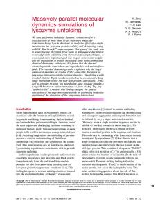
4 Nonbonded force calculation The GROMOS code approximates nonbonded forces by calculating them only for atom pairs which are within a certain cuto� radius of each other. As described in Section 5, these pairs are stored in a pair list which is updated in regular intervals. In the original code, this pairlist is represented by two arrays, INB and JNB. INB(I) gives the number of partners of atom I, and JNB can be thought of as a concatenation of lists of partners, one list for each atom. We also introduce the arrays firstJ and lastJ, so that the array section INB(firstJ(I) : lastJ(I)) gives the list of partners of atom I. Obviously, INB(I) = lastJ(I) ? firstJ(I) + 1 must hold. An important optimization in the sequential version is due to the fact that for each force exerted by an atom A on an atom B, atom B exerts an equal but opposite force on atom A. We therefore can cut the number of force calculations in half by storing each atom pair only once, for example by storing only partners with a higher atom index The resulting sequential version for N atoms is shown in Figure 1, where we assume that the force array F is initialized to 0 (similarly in the following code samples). Note also that in practice the force F and the positions X are vectors in IR3. In the IPfortran implementation [4], each processor executes the outer loop of the sequential version for a range (firstI(me) : lastI(me)) of atom indices. (Here, as throughout the text and the code samples,
DO I = 1, N DO J = rstJ(I), lastJ(I)
force = nbf(X(I) ? X(JNB(J))) F(I) = F(I) + force F(JNB(J)) = F(JNB(J)) ? force
ENDDO ENDDO
Figure 1: Sequential form of the nonbonded force calculation. me stands for the local processor id, which is accessible in IPfortran as thisnode and in Fortran D as my$proc. Similarly, P stands for the total number of processors, which is available as numnode and n$proc in the languages.) This range is determined in an initial call to a load balancing routine, of which gathering the corresponding portion of JNB, namely myJNB, is the most time consuming part. The code nishes with accumulating forces across processors, see Figure 2. Balance( rstI, lastI) DO I = rstI(me), lastI(me) DO J = rstJ(I), lastJ(I) force = nbf(X(I) ? X(myJNB(J))) F(I) = F(I) + force F(myJNB(J)) = F(myJNB(J)) ? force
ENDDO ENDDO F = +fFg
DECOMPOSITION AtomD(N, P), PairD(MP, P) DISTRIBUTE AtomD(*, BLOCK), PairD(*, BLOCK) ALIGN FF with AtomD, myJNB with PairD DO I = rstI(me), lastI(me) DO J = rstLocJ(I), lastLocJ(I)
force = nbf(X(I,me) ? X(myJNB(J,me))) FF(I,me) = FF(I,me) + force FF(myJNB(J,me),me) = FF(myJNB(J,me),me) ? force
ENDDO ENDDO FORALL I = 1, N FORALL ip = 1, P REDUCE(SUM, F(I), FF(I,ip)) ENDFORALL ENDFORALL
Figure 3: Force calculation, Fortran D version 1. MP is the maximal number of pairs per processor. done by replacing the global pairlist JNB with just portions thereof, myJNB. We then modeled that with our rst Fortran D version by adding an extra processor dimension. In our second Fortran D version now, we also use a two dimensional structure, JNBL, but now the second dimension does not represent a processor number, but a partner number instead. So, JNBL(I; :) represents all of the partners of atom I whose atom number is greater than I. We have
Figure 2: Force calculation, IPfortran version.
JNBL(I; 1 : INB(I)) = JNB(firstJ(I) : lastJ(I)):
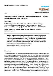
Note that this implementation replicates the force array F. A Fortran D version of this kind of algorithm can be written by expanding each array by one dimension (the processor dimension ), the introduced index being the processor number, and then distributing each array blockwise in that dimension. The resulting code is shown in Figure 3. However, this approach does not really take advantage of the Fortran D data distributions, since it ultimately limits our scalability. Instead of replicating the force array F, we should distribute it to distribute the workload. For allow load balancing, we distribute the data irregularly using a mapping array Map [8], which is determined by
We also guide the compiler by using a FORALL loop to indicate the fact that the operations are independent. The resulting code is shown in Figure 4.
DECOMPOSITION atomD(N), PartnD(N, MaxPD) DISTRIBUTE atomD(Map), PartnD(Map, *) ALIGN F WITH atomD, JNBL WITH PartnD FORALL I = 1, N ON HOME F(I) DO J = rstJ(I), lastJ(I) force = nbf(X(I) ? X(JNB(J))) F(I) = F(I) + force F(JNBL(I,J)) = F(JNBL(I,J)) ? force
ENDDO ENDFORALL
(*)
8I; 1 � I � N; 8p; 0 � p < P : firstI(p) � I � lastI(p) , Map(I) Figure=4:p:Force Calculation, Fortran D version 2. For enhanced locality, we combine that with an ON clause. We should also rethink how to distribute the neighbor list JNB as this represents the largest data structure of the problem. In the IPfortran version this was
It is worthwhile to aid our intuition about actual costs of computation and communication and about locality in general with some analysis. We start with de ning a predicate which indicates whether an atom
pair (I; K) is stored in the pairlist: � 9J, JNBL(I; J) = K, isPair(I; K) = 10 ifotherwise. We are also interested in how many force calculations involving atom K we have to perform on processor p: Partners(p; K) =
lastI X(p) I =firstI (p)
isPair(I; K):
For each processor p, we sum this up over all atoms: Pairs(p) = lastI X(p)
N X
I =firstI (p) K =1
N X
K =1
Partners(p; K) = lastI X(p)
isPair(I; K) =
I =firstI (p)
INB(I):
We notice that Pairs(p) is proportional to the computational load of processor p. Therefore, the overall computational cost is given by P P Tcomp / max Pairs(p) = max p=1 p=1
lastI X(p) I =firstI (p)
INB(I):
This is a typical load balancing problem [?], where the goal is N X Tcomp = Tideal / P1 � INB(I): i=1
This means that we have to choose firstI and lastI such that
has to make several contributions to F(I), it might be pro table to combine these contributions locally and then to just send the sum. While the assignments may be skewed for various reasons (for example, because only half of the pairs are stored, i.e., the pairlist satsi es JNBL(I; J) � I), we can estimate the average number of assignments which involve a particular atom simply by dividing by pairsave by N: ave Partnersave = INB P : Thus for P � INBave , we can expect every processor to contribute to most elements of F. On the other hand, for P � INBave , each processor contributes to very few elements of F. Therefore, the ratio Partners(ave) is crucial for the way we distribute F and how we perform the reduction operation. In the IPfortran version, F is replicated and all local contributions to an element of F are summed up locally. Then we globally combine the whole array, at the end all sums are everywhere available. Using a simple dimensional exchange, this summation can be done in O(N logP), with log P messages per processor (this works best for hypercubes, but can also be done on other parallel architectures). A more sophisticated divide-and-conquer approach works in O(N), with 2 logP messages per processor [7]. If we use the latter approach and have a balanced workload, then we have communication cost Tcomm / N and computation costs Tcomp / Pairsave . Thus it turns out that the ratio is Rcomp=comm = Partnersave=N = INBave =P;
which is again Partnersave. Thus for xed INBave , the cost of communication lastI X(p) N � INB ave will INB(I) � = Pairsave dominate for large P, independent of N. In the exPairs(p) = P periments with GROMOS parallelized in this way, for I =firstI (p) a system with N = 6968 atoms and INBave � 80, the cross-over point occurs near 128 processors on the Inholds (subscipts ave denote average values). tel iPSC860 (Figure 12). However, INBave increases After considering the raw computational costs, we cubicly in the cut-o� radius, so that the break-even now take a closer look at communication costs and, number of processors for which P / INBave inrelated to that, scalability. Most of the overall comcreases cubicly with the cut-o� radius as well. In the munication is associated with the potentially nonlocal limit of having an in nite cut-o� radius (that is, no assignment to the force array (statement (*) in Figcut-o� at all), we have INBave = N and the commuure 4). Compiling this na�vely, without message blocknication costs are swamped by the computational cost ing, would result in M1 � Pairsave (short) messages for any N � P: the algorithm is fully scalable as N per processor. For systems whose communicationtime increases. to send m units of data is well modeled by �+ m with � � [3], this would increase the communication cost [ This implementation is relatively communication by a factor �= . intensive in that the forces are not always computed Another issue besides raw message blocking is how locally. This avoids duplicate computations and is in much we can gain by combining non-local reductions. keeping with the spirit of the sequential algorithm. For example, if processor p does not own Atom I, but The experience with the GROMOS code parallelized
in this way [4] indicates that the communication overhead is tolerable for modest numbers of processors. However, for large numbers of processors, the cost of collecting F exceeds the cost of computing it in a distributed fashion. One way to achieve a scalable code for a xed cuto� radius is to allow each processor to compute all contributions to part of F, i.e., having JNB include all neighbors, not just those with larger atom index. This eliminates the assignment F(myJNB(J)) = F(myJNB(J)) ? force as well as the communication cost of F = +fF g, but at the expense of doubling the amount of computation. Note that doing the assignment F(JNBL(I; J)) = : : : on each iteration would still cause frequent communications to occur if compiled na�vely, without message blocking. This would increase the number of communications to an unacceptable level, on the order of Combined with recognition of the reduction operator by the compiler, the communication cost could be reduced to the same as (or even lower than) the previous algorithm by using a reduction like scatter add [2]. Based on this computation of Partnersave, let us now estimate the cost of communicating F. We assume that each processor is responsible for communicating Pairsave pieces of information. However, doing the reduction operations locally reduces the amount of communication by a factor Partnersave. When P � INBave , we expect Pairave � N. This means that, on average, each processor would need to communicate all of F, and thus the communication would be similar to the original algorithm. Thus the earlier comparison of computation versus communication cost applies in this case as well. The analysis is di�erent for P � INBave , where we expect Pairave � N and the communication cost becomes di�cult to predict. However, it does not appear necessarily to be an obstacle to scalability. Experimentation must be performed on actual data sets to determine the cost in practice. Note that as P increases, the size of blocked messages decreases, so the latency may have a detrimental e�ect. A route around the extra cost of communication is to duplicate computation of F. The serial code would be changed only by deleting the line F(JNB(J)) = F(JNB(J)) ? force; but we now must have the JNB array point to all neighbors, not just those with larger atom index. This of course doubles the amount of computation. However, such an increase might be tolerable in any case as indicated in the IPfortran example above, as it would
allow scalability in that case as well. In addition to distributing F one would also distribute JNB in order to avoid unnecessary duplication (recall JNB is the largest data structure in the problem, of size INBave � N). The complete Fortran D code is shown in Figure 5.
DECOMPOSITION atomD(N), PartnD(N, maxPD) DISTRIBUTE atomD(Map), PartnD(Map, *) ALIGN F WITH atomD, JNBL WITH PartnD DO I = 1, N DO J = 1, INB(I) F(I) = F(I) + nbf(X(I) ? X(JNBL(I,J))) ENDDO ENDDO Figure 5: Force Calculation, Fortran D version 3. We traded computation for communication. The version shown here distributes F and (following the owner computes rule) the workload regularly, i.e., without explicit load balancing. This can be improved on by using irregular distributions [6, 11]. ]
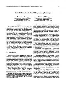
5 Pair-list generation Figure 6 shows the original version of the generation of the \pair list" JNB used in the nonbonded force calculation. The arrays firstI and lastI can J0 = 0 JJ = 0 DO I = 1, N DO J = I+1, N IF jX(I) ? X(J)j < R THEN JJ = JJ + 1 JNB(JJ) = J
ENDIF ENDDO
INB(I) = JJ ? J0 J0 = JJ
ENDDO
Figure 6: Pairlist computation, original version. be directly derived from INB. The critical obstacle for parallelizing this algorithm is the loop carried dependence on JJ, which causes a dependence for the assignment to JNB. However, the dependency does not occur in the values of JNB, but rather in the locations of the values. Thus we may compute each iteration separately and gure out later where to put them. By introducing the notion of a \scratch space"
JNBL we can easily remove the dependencies as in Figure 7. One di�culty in doing this automatically
DO I = 1, N JL = 0 DO J = I+1, N IF jX(I) ? X(J)j < R THEN JL = JL + 1 JNBL(JL,I) = J
ENDIF ENDDO INB(I) = JL ENDDO
1 � i � k, on the positions, xj , of atoms. Typically, this is extremely sparse, with i depending only on a small number of xj . Although the constraints are not linear (for example, they involve the distance between two points which includes expressions quadratic in the coordinates), any given constraint can be satis ed exactly by moving only one atom (with the others xed). Thus, the SHAKE algorithm iterates on i and moves a particular atom (say, atom number ji ) so that
i (x1 ; : : :; x^j ; : : :; xn) = 0. Since the previously computed values of xj are used, this can be viewed as a nonlinear Gauss-Seidel method. To make the analogy precise, consider a system of linear equations, i
.. .
DO I = 1, N JNB( rstJ(I):lastJ(I)) = JNBL(I, 1:INB(I)) ENDDO Figure 7: Pairlist computation, parallel-vector version. is that there is no a priori bound on the size of the scratch copies (i.e., how big we should declare the second dimension of JNBL). The above approach translates directly into the model needed in IPfortran. Each processor p will compute a range (firstI(p) : lastI(p)) of the iterations. The range sizes vary across processors due to the triangular shape of the double loop [4]. Each processor will have a (local) copy of part of the the JNB array. Since JNB is the largest data structure in the problem, it is likely that it would not ever be collected in one place, but rather it would be left distributed. However, it would be essential for load balancing to know the values of INB, which could be collected in IPfortran as in Figure 8. This exchange of information DO p = 0, n$proc?1 INB( rstI(p):lastI(p)) = INB( rstI(p):lastI(p)) @ p
ENDDO
Figure 8: Collect INB. is much less than optimal in terms of communication. An better approach in IPfortran that is better is described in the next section.
6 The SHAKE algorithm SHAKE utilizes a typical form of relaxation to solve a system of constraints regarding the distance (or angles) between particular atoms. Mathematically, there is a system of constraints, i (x1 ; : : :; xn) = 0,
ai1�1 + � � � + ain�n ? fi = 0; i = 1; : : :; n (think �i = xj and i � ai1 �1 + � � � +ain �n ? fi ). Then the i-th step of a Gauss-Seidel iteration is i
0 1 . X �i = @ aij �j ? fi A aii: j =i 6
It is well known that the Gauss-Seidel method does not parallelize well due to the fact that each step of the iteration depends on previous ones. A simple solution would be to use instead the Jacobi iteration �inew
0 1 . X = @ aij �j ? fi A aii; i = 1; : : :; n; old
j =i 6
followed by the assignment � new � old . This is now perfectly parallelizable, but is (usually) a more slowly convergent algorithm than Gauss-Seidel [9]. A typical solution is to introduce a compound algorithm for parallel computation which involves a Jacobi iteration across processors but interior to each processor, the Gauss-Seidel iteration is used. More precisely, the equations are partitioned into P sets, Ip, p = 0; : : :; P ? 1, and the iteration in each processor becomes
1 0 . X �i = @ aij �j ? fi A aii; i 2 Ip : j =i 6
At the completion of this, all processors exchange values of �j as necessary. Suppose that the sets Ip were the ranges 1 � j ? pn=P � n=P where for simplicity we assume n is an integer multiple of P. In IPfortran this can be written as in Figure 9. Note the global communication loop at the end, which runs in O(N) using divide and conquer [7]; a simple dimensional exchange would use time O(N logN).
much = n = P myslice = me * much
DO i = myslice+1, myslice+much XI(i) = 0.0 DO j = 1,n XI(i) = AMATRIX(i,j) * XI(j) ENDDO XI(i)= (XI(i)?F(i)) = AMATRIX(i,i) ENDDO
DECOMPOSITION CoordD(N) DISTRIBUTE CoordD(BLOCK) ALIGN X with CoordD much = n = P FORALL p = 0, P?1 myslice = p * much DO i = myslice+1, myslice+much XI(i) = 0.0 DO j = 1,n XI(i) = AMATRIX(i,j) * XI(j)
mask = 1 DO d = 1, CUBEDIM a = 1 + XOR(me, mask) * much * mask b = (1+XOR(me, mask)) * much * mask XI(a : b) = XI(a : b) @ p mask = 2 * mask
ENDDO XI(i)= (XI(i)?F(i)) = AMATRIX(i,i) ENDDO ENDFORALL
Figure 9: Hybrid relaxation: Gauss-Seidel locally, then Jacobi update globally. IPfortran version.
tion are given. The dominating parts of the sequential algorithm, the nonbonded forces and pair list, have been parallelized with nearly perfect speedup. Time-stepping and the bonded force calculation, performed redundantly at every processor, remain constant. These, together with the load balancing and global sum of the nonbonded force, form an asymptote which the total time approaches as the number of processors is increased. As the problem size, N, is increased, the pair list construction (and long-range force calculation, included in this section of the timing) grows as O(N 2 ); all other parts increase by O(N), with the exception of the load balancing which is dependent on both initial data and time and, relative to this discussion, is di�cult to characterize. Thus we can assert that this simple port of the GROMOS code is scalable. Increasing the cuto� radius while keeping N xed also increases the number of processors that can be used e�ectively, as discussed in Section 4, thereby shifting the nonbonded force curve up by some delta.
ENDDO
much = n = P
DO ip = 0, P?1 myslice = ip * much DO i = myslice+1, myslice+much XI(i) = 0.0 DO j = 1, n XI(i) = AMATRIX(i,j) * XI(j) ENDDO XI(i) = (XI(i)?F(i)) = AMATRIX(i,i) ENDDO ENDDO Figure 10: Hybrid relaxation, Fortran D version 1. When coding SHAKE in Fortran D, it is tempting to write the code in Figure 10, but this is just GaussSeidel in a more complex form, since in the innermost loop we reference all of J. As it turns out, there is no simple sequential algorithm that can be annotated to yield the above hybrid relaxation. However, using the Fortran D FORALL loop we achieve the desired semantics, see Figure 11.
7 Performance results Figure 12 gives performance results for the parallel implementation of GROMOS using IPfortran. The calculation on an Intel iPSC/860 uses a model for the enzyme Superoxide Dismutase [18], with a total of 6968 atoms, for 500 timesteps. Execution times for both the overall and principal sections of the calcula-
Figure 11: Hybrid relaxation, Fortran D version.
8 Conclusions Because this study was limited to a single example program and two languages, we cannot make broad generalizations regarding parallel programming. However, GROMOS as we have implemented it uses only straight-forward implementations of fundamental computational molecular dynamics algorithms. We therefore believe that the following observations will apply to a range of those codes. � Both local and global models are feasible interfaces for programming distributed-memory parallel machines. This agrees with previous
Time in minutes
103
102
101
100
10-1 . 100
o
o o
o
o
o
o
o
o o
o
o
o
o
o o
o o
o
o o o
o
o
o
o
o
total iPSC/860
shake (time-stepping) nonbonded force (nbf) pairlist bonded force
global sum nbf load balancing
102
Parallel GROMOS: 500 steps, 6968 atoms
o
o o
o
o
o
o
101 Number of processors
.
103 Figure 12: Performance results. work [17]. In addition, both models can provide the user with a higher-level programming interface than current message-passing languages on distributed-memory machines.
� Regardless of the implementation model chosen,
the key to a good parallel program is the choice of an appropriate algorithm. This implies that programs will have to be rewritten to some extent for parallelization, rather than relying on compiler optimization of \dusty deck" code. This resembles the development of a \vectorizable style" of programming vector architectures [20]. In the parallel arena, the equivalent challenge is the development of a \machine-independent parallel programming style," a long-term research target of Fortran D [12].
� IPfortran improves on the usual message-passing
environment by eliminating the need for explicit \send" operations. This simpli es code signi cantly, allowing the programmer to concentrate on higher-level problems such as load balancing. The local model of computation is also convenient for some algorithms which have distinct \on-processor" and \inter-processor" phases.
� Fortran D abstracts all communication out of the
program by providing a modi ed shared-memory model of computation. The key feature of a Fortran D program is the data distribution, which the compiler uses to generate the low-level communications operations. [ This is meant to be
nearer to the original sequential Fortran model of computation. Our experiments indicate this may be the case for some algorithms, but not for some explicitly parallel algorithms. ] � Achieving scalability in molecular dynamics, requires careful algorithm design, but is an achievable goal. We plan to continue this work in several areas. Both the IPfortran and Fortran D implementations will continue to go forward, and the lessons from this study and others like it will a�ect their development. In the computational molecular dynamics area, we will continue to design and implement scalable algorithms, producing high-performance codes [6][HPF ref Chuck???]. Finally, we plan to pursue research into other methods of data partitioning for this problem and in more general settings. To do: 1. clean up bibliography (HPF ref, JPDC issue number).
References [1] Babak Bagheri, Terry W. Clark, and L. Ridgway Scott. IPfortran (a parallel extension of Fortran) reference manual. Research Report UH/MD{119, Dept. of Mathematics, University of Houston, 1991. [2] H. Berryman, J. Saltz, and J. Scroggs. Execution time support for adaptive scienti c algorithms on distributed memory machines. Concurrency: Practice and Experience, 3(3):159{178, June 1991. [3] D. K. Bradley. First and second generation hypercube performance. Technical Report UIUCDCS{R{88{1455, Dept.
[4] [5] [6] [7] [8]
[9]
[10] [11]
[12] [13] [14] [15] [16] [17] [18] [19] [20]
of Computer Science, University of Illinois at UrbanaChampaign, 1988. Terry W. Clark, J. A. McCammon, and L. Ridgway Scott. Parallel molecular dynamics. In Proceedings of the Fifth SIAM Conference on Parallel Processing for Scienti c Computing, Houston, TX, March 1991. Terry W. Clark and J. Andrew McCammon. Parallelization of a molecular dynamics non-bonded force algorithm for mimd architecture. Computers & Chemistry, 14(3):219{224, 1990. Terry W. Clark, Reinhard v. Hanxleden, and L. Ridgway Scott. Scalable algorithms for molecular dynamics computations. Technical report, Dept. of Mathematics, University of Houston, to appear. G. C. Fox, M. Johnson, G. Lyzenga, S. Otto, J. Salmon, and D. Walker. Solving Problems on Concurrent Multiprocessors. Prentice-Hall, 1988. Geo�rey Fox, Seema Hiranandani, Ken Kennedy, Charles Koelbel, Uli Kremer, Chau-Wen Tseng, and Min-You Wu. Fortran D language speci cation. Technical Report TR90141, Dept. of Computer Science, Rice University, December 1990. Revised April, 1991. Girija Ganti and J. Andrew McCammon. Transport properties of macromolecules by brownian dynamics simulation: Vectorization of brownian dynamics on the Cyber205. Journal of Computational Chemistry, 7(4):457{463, 1986. W. F. van Gunsteren and H. J. C. Berendsen. GROMOS: GROningen MOlecular Simulation software. Technical report, Laboratory of Physical Chemistry, University of Groningen, Nijenborgh, The Netherlands, 1988. Reinhard v. Hanxleden and Ken Kennedy. Relaxing SIMD control ow constraintsusing loop transformations. In Proceedings of the ACM SIGPLAN '92 Conference on Program Language Design and Implementation, San Francisco, CA, 1992. S. Hiranandani, K. Kennedy, C. Koelbel, U. Kremer, and C. Tseng. An overview of the Fortran D programming system. Technical Report TR91-154, Dept. of Computer Science, Rice University, March 1991. C. A. R. Hoare. Communicating Sequential Processes. Prentice-Hall, Englewood Cli�s, NJ, 1985. C. Lin and L. Snyder. A comparison of programming models for shared memory multiprocessors. In Proceedings of the 1991 International Conference on Parallel Processing, Vol. 2, pages 163{170, 1991. J. Andrew McCammon. Computer-aidedmolecular design. Science, 238:486{491, October 1987. J. Andrew McCammon and Stephen C. Harvey. Dynamics of proteins and nucleic acids. Cambridge University Press, Cambridge, 1987. L. R. Scott, J. M. Boyle, and B. Bagheri. Distributed data structures for scienti c computation. In M. T. Heath, editor, Proceedings of the 3rd Hypercube Multiprocessors Conference, pages 55{66, Philadelphia, PA, 1987. Jian Shen and J. Andrew McCammon. Molecular dynamics simulation of superoxide interacting with superoxide dismutase. Chemical Physics, 158:191{198, 1991. R. van de Geijn. On global combine operations. LAPACK Working Note 29. Michael J. Wolfe. Semi-automatic domain decomposition. In Proceedings of the 4th Conference on Hypercube
Concurrent Computers and Applications, Monterey, CA, March 1989.