Evaluating the Impact of Improvements in the Boundary Layer ...

3136

MONTHLY WEATHER REVIEW

VOLUME 143

Evaluating the Impact of Improvements in the Boundary Layer Parameterization on Hurricane Intensity and Structure Forecasts in HWRF JUN A. ZHANG NOAA/AOML/Hurricane Research Division, and Cooperative Institute for Marine and Atmospheric Studies, University of Miami, Miami, Florida

DAVID S. NOLAN Rosenstiel School of Marine and Atmospheric Science, University of Miami, Miami, Florida

ROBERT F. ROGERS NOAA/AOML/Hurricane Research Division, Miami, Florida

VIJAY TALLAPRAGADA NOAA/NWS/NCEP/Environmental Modeling Center, College Park, Maryland (Manuscript received 14 October 2014, in final form 2 April 2015) ABSTRACT As part of the Hurricane Forecast Improvement Project (HFIP), recent boundary layer physics upgrades in the operational Hurricane Weather Research and Forecasting (HWRF) Model have benefited from analyses of in situ aircraft observations in the low-level eyewall region of major hurricanes. This study evaluates the impact of these improvements to the vertical diffusion in the boundary layer on the simulated track, intensity, and structure of four hurricanes using retrospective HWRF forecasts. Structural metrics developed from observational composites are used in the model evaluation process. The results show improvements in track and intensity forecasts in response to the improvement of the vertical diffusion. The results also demonstrate substantial improvements in the simulated storm size, surface inflow angle, near-surface wind profile, and kinematic boundary layer heights in simulations with the improved physics, while only minor improvements are found in the thermodynamic boundary layer height, eyewall slope, and the distributions of vertical velocities in the eyewall. Other structural metrics such as warm core anomaly and warm core height are also explored. Reasons for the structural differences between the two sets of forecasts with different physics are discussed. This work further emphasizes the importance of aircraft observations in model diagnostics and development, endorsing a developmental framework for improving physical parameterizations in hurricane models.

1. Introduction The Hurricane Forecast Improvement Project (HFIP) has provided an opportunity for the National Oceanic and Atmospheric Administration (NOAA) and other agencies to coordinate hurricane research required to substantially advance hurricane track and intensity forecasts (Gall et al. 2013). The most difficult challenge of reaching the goals of

Corresponding author address: Jun A. Zhang, NOAA/AOML Hurricane Research Division, 4301 Rickenbacker Causeway, Miami, FL 33149. E-mail: [email protected] DOI: 10.1175/MWR-D-14-00339.1 Ó 2015 American Meteorological Society

HFIP has been in improving hurricane intensity forecasts. Hurricane intensity is controlled by processes both external and internal to the storm (e.g., Marks and Shay 1998; Rogers et al. 2006, 2013a). The external processes are controlled by the large-scale flow surrounding the hurricane (e.g., Molinari et al. 1995; Bosart et al. 2000; Kaplan and DeMaria 2003; Dunion and Velden 2004; Braun 2010; Kaplan et al. 2010). Improving model representation of large-scale processes controlling intensity requires improvements in global models. On the other hand, the internal processes are controlled by axisymmetric and asymmetric vortex-scale, convective-scale, and turbulent processes occurring within the hurricane, particularly in

AUGUST 2015

ZHANG ET AL.

or near the eyewall, and by the interaction with the ocean (e.g., Emanuel 1995; Schubert et al. 1999; Kossin and Eastin 2001; Montgomery et al. 2006, 2014; Nolan et al. 2007; Reasor et al. 2009; Rogers 2010; Riemer et al. 2010; Cione et al. 2013). The spatial scales of these processes typically are on the order of 1–10 km, and even smaller in the boundary layer. As a result, improvements in model simulation of internal processes controlling intensity require advancement of higher-resolution regional models. As part of HFIP, Zhang et al. (2012) presented a model development framework for improving the physical parameterizations using quality-controlled and postprocessed aircraft observations. This framework consists of four main steps: 1) model diagnostics, 2) physics development, 3) physics implementation, and 4) further evaluation. While Zhang et al. (2012) focused on demonstrating the usefulness of the first three steps of this framework, this study concentrates on the fourth step to further validate this framework through model diagnostics of real-case hurricane simulations. This further evaluation aims to verify the success of the first three steps and more importantly to identify remaining deficiencies in the simulations. Here we show that this framework is successful in improving the boundary layer physics of the Hurricane Weather Research and Forecasting (HWRF) Model, providing a path to guide continued model development for HWRF as well as other hurricane models. Using idealized simulations, Gopalakrishnan et al. (2013) showed that the above-mentioned framework is potentially successful for improving the surface layer and boundary layer parameterization schemes in HWRF. They studied the impact of vertical diffusion (Km) on simulated hurricane intensity and structure. They found that reducing Km has a significant influence on hurricane size and boundary layer height. Tallapragada et al. (2014) reported on recent upgrades in the 2012 HWRF that include a new higherresolution nest, improved vortex initialization, improved boundary layer physics, and some critical bug fixes, and they documented the impacts of these combined upgrades on track and intensity forecasts. Using retrospective forecasts from the 2011–12 hurricane seasons, they found significant improvements in the track and intensity forecasts in the 2012 HWRF as compared to the 2011 HWRF. They also found dramatic improvements in the verification of storm size in terms of wind radii at 34-, 50-, and 64-kt (1 kt 5 0.5144 m s21) thresholds in different quadrants. Finally, they found that the relationship between minimum sea level pressure and maximum 10-m wind is improved in the 2012 HWRF as compared to the previous versions, suggesting the dynamics in HWRF was improved. They attributed the improvements in the simulated storm size mainly to improved vortex initialization and the higher horizontal resolution that allows the model to resolve the

3137

inner core of TCs more accurately. However, Tallapragada et al. (2014) did not evaluate the individual impact of each component of the improvements made in the 2012 HWRF on track, intensity, and structure predictions. The present paper aims to evaluate the impact of one component of the 2012 HWRF upgrade—the boundary layer physics modification—on forecasts of track, intensity, and structure, with an emphasis on model evaluation using structural metrics compared to aircraft observations. Through comparisons of the structural metrics derived from model outputs and observational composites, we aim to verify and advance the findings from previous idealized HWRF simulations (i.e., Gopalakrishnan et al. 2013). We also aim to provide feedback for the HWRF model developers as to how the simulated structure was improved by the upgraded PBL physics alone and what model deficiencies may remain after the physics upgrade. The traditional verification parameters of the National Hurricane Center include the mean absolute errors and biases of their deterministic forecasts of track and maximum wind speed. These are useful metrics for monitoring long-term trends of forecast capability, but they provide little insight into the causes of the errors or how the models might be improved. Thus, it is helpful to develop diagnostic techniques and metrics to enhance model verification. In particular, physically based analyses of hurricane forecast models will help improve the understanding of model behavior and provide guidance for model improvements. In this study, we utilize structural metrics including storm size (i.e., the radius of maximum wind speed), inflow angle of the surface wind, boundary layer heights, eyewall slope, and statistics of eyewall vertical velocity w. In addition, we emphasize the importance of using the compositing method to conduct model diagnostics. The advantage of the compositing methodology is that the skills of the numerical models can be evaluated in a statistical sense. Model deficiencies can be identified through comparing model and observational composites with more confidence than using a case study approach. At the same time, model improvements can be recognized through comparing model simulations before and after model upgrades against observations. By showing a case with model evaluation and improvement of a specific model (e.g., HWRF) and one aspect of physics upgrade (e.g., boundary layer), we aim to demonstrate that the methodology used here can be adapted by the research community for evaluating and improving other aspects of the model physics in different types of numerical models. Here we also show that improving simulated storm structure is associated with improvements in intensity forecasts. Section 2 gives a brief summary of the observational data and model simulations used in this work as well as the analysis method; section 3 presents the impact of

3138

MONTHLY WEATHER REVIEW

VOLUME 143

boundary layer physics upgrades on the track and intensity forecasts, and presents evaluation of the impact of the physics upgrades on the simulated structures; section 4 discusses possible reasons for the structural differences seen in the model diagnostics; and section 5 summarizes our results.

2. Model simulations, observations, and analysis method The HWRF system was developed at NOAA’s National Weather Service (NWS) and became an operational hurricane model in 2007. An experimental version of the HWRF system (dubbed ‘‘HWRFX’’) was developed at NOAA’s Hurricane Research Division (HRD). HWRFX was developed to operate both in an idealized and real-storm framework (Gopalakrishnan et al. 2011, 2012). The 3-km HWRFX model (X. Zhang et al. 2011) was recently merged with the operational HWRF (i.e., HWRFV3.2), which is currently used by NOAA for operational hurricane forecasting. As described by Gopalakrishnan et al. (2013) and Tallapragada et al. (2014), physics upgrades in the operational HWRF were made based on comparisons to observations. The boundary layer scheme used in HWRF is essentially the traditional medium-range forecast (MRF) scheme (Troen and Mahrt 1986; Hong and Pan 1996). It is called the ‘‘GFS scheme’’ in the HWRF community (e.g., Gopalakrishnan et al. 2013; Tallapragada et al. 2014). In this scheme, turbulent fluxes are parameterized using the vertical eddy diffusivity and the vertical gradient of the mean quantities. For instance, the momentum flux or wind stress t is parameterized as (1)

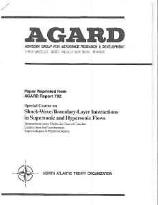
FIG. 1. Comparison of vertical eddy diffusivity Km between model simulations and observations at 500 m. Boundary layer schemes as in the (a) 2011 and (b) 2012 versions of the HWRF Model are shown. This figure is reproduced from Zhang et al. (2012). Observations are shown by the blue 3, which are from J. A. Zhang et al. (2011a).

where r is the air density, u is the wind speed, and Km is the vertical eddy diffusivity. In the boundary layer scheme, Km is parameterized in the form of

given by J. A. Zhang et al. (2011a). During the physics upgrade, a parameter a was added to Eq. (2) to control the magnitude of Km as follows:

Km 5 k(u*/F)z(1 2 z/h)2 ,

Km 5 k(u*/F)z[a(1 2 z/h)2 ] .

t/r 5 Km ›u/›z,

(2)

where k 5 0.4 is the Von Kármán constant, u* is the surface frictional velocity, F is the stability function evaluated at the top of the surface layer, z is the height above the surface, and h is the depth of the turbulent PBL (also known as the mixed layer) that is determined based on the height above the ground at which the bulk Richardson number exceeds a critical value. Before the boundary layer physics upgrade, deficiencies in simulated boundary layer structure were identified in our previous work as part of HFIP’s High Resolution Hurricane (HRH) test (Zhang et al. 2012). Very large values of Km were produced in versions prior to 2011 (Fig. 1a) compared to observations

(3)

Note that when a 5 1, Eq. (3) is equivalent to Eq. (2). As noted by Zhang et al. (2012) and Gopalakrishnan et al. (2013), a 5 0.25 matches best with observations of Km in idealized HWRF simulations. In the 2012 version of the operational HWRF,1 a was set to 0.5 based on extensive tests conducted using retrospective simulations of all the storms in the 2010–11 seasons (Tallapragada et al. 2014). Figure 1b compares Km used in the 2012 HWRF in comparison with observations. 1 Note that upgrades are made to HWRF on a regular schedule every year, so HWRF is usually different from year to year.

AUGUST 2015

ZHANG ET AL.

3139

TABLE 1. Summary of storm information and HWRF simulations. Storm name

No. of cycles of simulations

Starting time of the first cycle

Starting time of the last cycle

Bill Earl Karl Irene

33 40 15 34

1800 UTC 15 Aug 2009 1800 UTC 25 Aug 2010 1800 UTC 14 Sep 2010 1800 UTC 20 Aug 2011

1800 UTC 23 Aug 2009 1200 UTC 4 Sep 2010 0600 UTC 18 Sep 2010 0000 UTC 29 Aug 2011

Surface layer physics upgrades were made in 2010 by modifying the exchange coefficient for enthalpy transfer (Ck) based on recent observations given by Zhang et al. (2008) and Haus et al. (2010). In the surface layer scheme of HWRF, over the ocean, the drag coefficient (Cd) under the neutral condition is parameterized through the surface roughness length (z0) in the form of "

k Cd 5 ln(10/z0 )

#2 .

(4)

Here z0 is parameterized a function of the wind speed u at 10 m as follows: z0 5 (0:0185/g) 3 (7:59 3 1028 u2 1 2:46 3 1024 u)2 , u # 12:5 m s21 ,

(5)

z0 5 (7:40 3 1024 u 2 0:58) 3 1023,

12:5 , u # 30 m s21, (6)

z0 5 21:34 3 10

24

2 3:57 3 10

25

1 3:02 3 10

28 3

u 1 1:52 3 10

u 2 2:05 3 10

210 4

u ,

26 2

u

u . 30 m s21, (7)

where g 5 9.81 m s22 is the gravitational acceleration. Two sets of HWRF forecasts using 1) the PBL scheme as in the 2012 operational HWRF model (referred to as PBL12 hereafter), and 2) the PBL scheme from the 2011 version HWRF, using the larger value of Km (PBL11 hereafter), were conducted with the same initial and boundary conditions. All other physics packages are the same for the two sets of forecasts except the parameterization of Km as discussed above. For the purpose of evaluating only the impact of PBL physics, forecasts used for both PBL11 and PBL12 composites were performed with 3-km horizontal resolution for the inner nest. A total of 122 forecasts of 4 hurricanes (Hurricanes Bill, Earl, Karl, and Irene) were conducted using PBL11 and PBL12.2 These forecasts were generated in a cycling mode every 6 h in the same manner as in the operational

2 These storms are chosen mainly because there are good observational data coverage for these storms.

HWRF forecasts (Tallapragada et al. 2014). Each cycle generates a 5-day forecast with hourly output. The number of cycles for each storm depends on its lifetime. Table 1 summarizes the storm information along with the number of cycles of simulations and starting time of the first and last cycles. The observed tracks of these four hurricanes are shown in Fig. 2. The observational data used for model evaluation are composites of a large number of GPS dropsonde and Doppler radar data from multiple storms. Different aspects of these composite structures (including vortexand convective-scale, boundary layer, and surface layer) were documented in detail by J. A. Zhang et al. (2011b), Zhang and Uhlhorn (2012), and Rogers et al. (2012). In our composite framework, data are grouped as a function of the radius to the storm center r normalized by the radius of maximum wind speed; that is, r* 5 r/RMW, where RMW is defined as the radius of maximum axisymmetric wind speed at 2 km. The center positions have been computed using the flight-level data to fix the storm center with the algorithm developed by Willoughby and Chelmow (1982). In addition, the eyewall slope data from Stern and Nolan (2009) with updated Doppler radar observations (Stern et al. 2014) in multiple storms are used. We composite model simulations in the same framework as in the observational composite analysis (e.g., for axisymmetric structure comparison, the model outputs were azimuthally averaged and presented as a function of the height and radial distance normalized by RMW).

FIG. 2. Best tracks of Hurricane Bill (2009), Earl (2010), Karl (2010), and Irene (2011).

3140

MONTHLY WEATHER REVIEW

FIG. 3. Plots of absolute errors of (a) track and (b) intensity forecasts, and (c) intensity bias from the two sets of HWRF forecasts with PBL11 and PBL12 of four hurricanes listed in Table 1.

Only category 1 and stronger storms are selected from the 122 forecasts in the composite analysis. A total of ;7000 h of forecasts are used in the analysis.

3. Results The absolute errors of track and intensity forecasts as well as the intensity bias for PBL11 and PBL12 are shown in Fig. 3, which were derived by comparing the simulated track and intensity to the best track data from the National Hurricane Center (NHC). The number of cases in the above verification every 12 h is also plotted. It appears that the track forecast is very slightly improved in the PBL12 composite compared to the PBL11 composite (Fig. 1a). On the other hand, the intensity forecast is noticeably improved (;5% on average) from PBL11 to PBL12, especially before 72 h. The bias in the intensity forecast is also reduced (Fig. 3c). The frequency distribution of the storm intensities from both sets of forecasts and the best track (Fig. 4) also indicate an improved distribution of intensity forecasts for PBL12 compared to PBL11. On average storms in the PBL12 forecasts are stronger than those in the PBL11 forecasts. Note that the improvements in track and intensity forecasts here are purely due to the improvement of the PBL physics. In the verification of the 2012 version of HWRF

VOLUME 143

FIG. 4. Frequency distributions of storm intensity for HWRF forecasts with (a) PBL11, (b) PBL12, and storm intensity from (c) the best track.

compared to the 2011 version reported recently by Tallapragada et al. (2014), the improvements in track (;19%) and intensity (;10%) forecasts also included the effect of increasing model horizontal resolution from 9 to 3 km for the finest nest. As mentioned earlier, the goal here is to evaluate the impact of improvements in the boundary layer parameterization on simulated intensity and structure separately from the improvements in model horizontal resolution. Figure 5 shows the frequency distribution of the RMW at 10 m for the PBL11 and PBL12 composites. It clearly demonstrates that the mean size of the simulated storms in the PBL11 composite is substantially larger than that in the PBL12 composite, with a mean difference of ;10 km. Estimates of RMW from the Stepped Frequency Microwave Radiometer (SFMR) data in these storms showed the mean RMW for these four storms3 to be ;37 km. The PBL12 composite values (mean ;44 km) are closer to the observations than the PBL11 composite values (mean ;53 km), indicating that the PBL12 physics improves 3 Only forecast times where there are SFMR data are used in the analyses.

AUGUST 2015

ZHANG ET AL.

3141

FIG. 6. Plot of surface inflow angle as a function of radius to the storm center normalized by the radius of maximum wind speed for the PBL11 and PBL12 composites. Observations are from Zhang and Uhlhorn (2012).

FIG. 5. Frequency distributions of simulated radius of maximum wind speed at 10 m for HWRF forecasts with (a) PBL11, (b) PBL12, and (c) observations. The observed RMWs are estimated using the Stepped Frequency Microwave Radiometer (SFMR) data.

forecasts of storm size. Our result is different from that given by Bryan (2012), who found in axisymmetric numerical simulations that the RMW (at either the surface or 2-km height) did not seem to have a systematic dependence on vertical diffusivity (by varying the mixing length). However, Bryan’s simulations usually lasted for 12 days and thus could reach an equilibrium state in which the storm size may be controlled by many different factors. The surface inflow angle represents the relative strengths of the radial (Vr) and tangential (Vt) wind velocities at the ocean surface. Since air parcels move from the ambient region to the storm center following the inflow trajectory, how the inflow angles vary with distance to the storm center is tied to the energy exchange near the air–sea interface. Here we compare the radial distribution of surface inflow angles for the PBL11 and PBL12 composites and compare the composite results with observations based on the GPS dropsonde data as reported by Zhang and Uhlhorn (2012). Note that here the entire observational dataset of Zhang and Uhlhorn (2012) are used in the comparison. Figure 6 illustrates that the simulated surface inflow angle and its radial variation in the PBL12 composite is much closer to the observations than those in the PBL11 composites. In particular, the magnitude of the

surface inflow angle is substantially improved in PBL12 compared to PBL11. Note that the biases in the surface inflow angle in PBL11 are mainly due to the errors in Vr compared to observations.4 The radial variation of the surface inflow angle in both PBL11 and PBL12 composites is different from the observed radial variation. While the observations show a strongly peaked inflow angle near r* 5 1.75, both PBL11 and PBL12 show smother variations with a maximum inflow angle closer to r* 5 1.5. One metric used by Kepert (2012) to validate boundary layer simulations is the shape of wind profile in the surface layer. According to traditional Monin–Obukhov similarity theory, the surface layer wind speed should follow the logarithmic relationship with height if turbulent fluxes are constant with height in the surface layer under neutral stability conditions. Zhang and Drennan (2012) verified that turbulent fluxes tend to be nearly constant in the surface layer between the rainbands, at surface winds between 20 and 30 m s21, using directly measured flux data collected during the Coupled Boundary Layers Air–Sea Transfer (CBLAST) experiment (Black et al. 2007; Zhang et al. 2008). Figure 7 compares the vertical wind profiles in the layer from the lowest model level (;30 m) to 600 m for four radial locations (r* 5 1, 1.5, 2, and 2.5) from the PBL11 and PBL12 composites. Mean wind profiles from the dropsonde composite of J. A. Zhang et al. (2011b) are also shown. It appears that the wind speed increases with height more quickly in the PBL12 composite than in the 4 The azimuthal 10-m Vr is on average 2–7 m s21 weaker in PBL11 than that in PBL12 and the dropsonde composite.

3142

MONTHLY WEATHER REVIEW

VOLUME 143

FIG. 7. Plots of vertical wind profiles in the layer between the lowest model level and 600 m from the PBL11 and PBL12 composites at radial locations (a) r* 5 1, (b) r* 5 1.5, (c) r* 5 2, and (d) r* 5 2.5. The mean wind profile from the dropsonde composite of J. A. Zhang et al. (2011b) is also shown. The green dashed lines are the wind profiles calculated using the slope u*/k as a function of height in log scale.

PBL11 composite, indicating the near-surface vertical wind shear is stronger in PBL12. The observed wind profiles have relatively larger wind shear and are quantitatively closer to those in the PBL12 composite. Smith and Montgomery (2014) argued that the logarithmic surface layer does not exist for the hurricane core (i.e., eyewall region). This argument may be valid for heights below 50 m assuming the errors in the wind profile from dropsonde composite are small.5 However, the lowest model level in HWRF is above ;35 m. Both model simulations and observations indicate a logarithmic wind profile above the lowest model level. J. A. Zhang et al. (2011b) studied boundary layer height scales in hurricanes using hundreds of GPS dropsonde profiles. Through compositing the profiles, 5

Testing if the departure of the wind profile from the log law is larger than the expected measurement uncertainty including turbulence is beyond the scope of this study.

they found that there are different height scales that can be used to define the top of the boundary layer. These height scales include the height of the maximum tangential wind speed (hvtmax), the depth of the inflow layer defined as the height of 10% peak inflow (hinflow), and the thermodynamic mixed layer depth defined either as 1) the height where the difference of virtual potential temperature (uy) and the mean of uy over the lowest 150 m equals 0.5 K (Zid), or 2) the vertical gradient of uy equals 3 K km21 (Zig). Here we evaluate these four boundary layer height scales in the model composites from PBL11 and PBL12. Azimuthally averaged fields will be presented as a function of radius normalized by RMW (r* 5 r/RMW) and of dimensional height z. To get meaningful comparisons in hvtmax and hinflow, we normalized Vt and Vr by their maximum values in both the PBL11 and PBL12 composites. Figures 8a, 8b, and 8c show Vt normalized by the maximum value of Vt as a function of r* and z for PBL11,

AUGUST 2015

ZHANG ET AL.

3143

FIG. 8. Plots of (a)–(c) tangential wind and (d)–(f) radial wind as a function of r/RMW and height. (top) PBL11, (middle) PBL12, and (bottom) the dropsonde composites from J. A. Zhang et al. (2011b). The dashed line represents the height of the maximum tangential wind speed and the solid line represents the inflow layer depth defined as the height of 10% peak inflow. White lines show the estimates of boundary layer height based on linear hurricane boundary layer theory.

PBL12, and sonde composites, respectively, from J. A. Zhang et al. (2011b). The dashed line in each panel represents hvtmax. The white line represents the boundary layer height scale h based on hurricane boundary layer theory (Kepert 2001; Kepert and Wang 2001) that relates h to Km and inertial stability I in the form of h 5 (2Km /I)1/2 .

(8)

Note that for the observational composite, Km used for calculation of the theoretical h was obtained by fitting a linear function to the observed Km shown in Fig. 1. It appears that hvtmax in the PBL12 composite is much closer to observations than that in the PBL11 composite. Near the eyewall region (r* 5 1), the observed hvtmax is ;600 m, but hvtmax in the PBL11 composite is ;1000 m while it is ;600 m in the PBL12 composite. Second, both

3144

MONTHLY WEATHER REVIEW

PBL11 and PBL12 forecasts capture the trend of decrease of hvtmax with decreasing radius, especially close to the eyewall region. This behavior is captured in the PBL12 composite across a greater radial distance than in the PBL11 composite (i.e., r* , 1.8 in PBL12 vs r* , 1.2 in PBL11). In the outer radii (1.5 , r* , 2.5), hvtmax in the PBL12 composite is much higher than that observed, which is a remaining model deficiency. Figures 8d, 8e, and 8f show Vr (normalized by its maximum absolute value) as a function of r* and z for PBL11, PBL12, and sonde composites, respectively. The solid line in each panel shows the inflow layer depth (hinflow). The theoretical boundary layer height scale is shown by the white line. The result for hinflow is similar to that of hvtmax, with hinflow in the PBL12 composite being much closer to observations. Around the eyewall region (r* ; 1), the observed hinflow is ;800 m, but hinflow in the PBL11 composite is ;1200 m, which is substantially deeper than that in the PBL12 composite and the observed value. Both PBL11 and PBL12 composites captured the observed trend of decreasing hinflow with decreasing radius. Both composites also captured the feature of hvtmax being within the inflow layer. It is found also that hinflow in the outer radii (r* . 1.5) is higher for both PBL11 and PBL12 composites than that in the dropsonde composite.6 At the eyewall region (r* ; 1), hinflow is found to be ;2h in the PBL12 and dropsonde composites, however, hinflow is much closer to h (hinflow ; 1.3h) in the PBL11 composite. Kepert (2010b) found that hinflow ; 2.5h in the linear hurricane boundary layer model. The radial gradient of hinflow in the eyewall region is much larger in the model composites than in the observational composite. We also note that the lack of outflow in the model simulation, and the weak vertical shear of the azimuthal wind above 1-km height, suggesting that the mixing may be a bit too strong in this region even after the physics upgrade. This is also consistent with the fact that Km at large wind speeds is still greater than what the observations indicate (cf. Fig. 1). Figure 9 shows the comparison of the thermodynamic mixed layer depths between the PBL11 and PBL12 composites as well as observations. As mentioned earlier, two types of calculations of the mixed layer depth are tested. Figures 9a, 9b, and 9c show the difference (uy2diff) between uy and the mean uy of the lowest 150 m (uy150) as a function of r* and z for PBL11, PBL12, and dropsonde composites, respectively. Figures 9d, 9e, and 9f show the vertical gradient (or lapse rate) of uy as a function of r* and z, for PBL11, PBL12, and dropsonde

VOLUME 143

composite, respectively. The solid line indicates the mixed layer depth as defined for each variable. Figure 9 indicates that the simulated uy2diff and the lapse rate are generally similar between the PBL11 and PBL12 composites. Both sets of the HWRF forecasts captured the trend of decreasing mixed layer depth with decreasing radius. The difference in uy2diff is quite small between the PBL11 and PBL12 composites. The simulated uy2diff in the two composites is also consistent with observations in term of the magnitude. The difference is mainly in the radial variation of uy150 inward from the eyewall, showing that the radial gradient of uy150 at r* ; 0.75 is much sharper in the simulations than in observations. Note that the small radial gradient in the dropsonde composite may be due to the artifact of the low horizontal resolution of the data.7 The magnitude of the lapse rate of uy is generally similar in the two composites and the observations (Figs. 9d–f). The PBL12 composite captures the stronger stable layer inside the eyewall and above 1 km, which is more consistent with observations than the PBL11 composite. Near the surface, the PBL12 composite also simulates a slightly more unstable layer outside of r* 5 1 than the PBL11 composite, again more consistent with observations. The profiles of Zid and Zig in the PBL11 and PBL12 composites are similar, with the PBL12 composite profile being slightly shallower (;30 m) in the eyewall region. This result indicates that there is only very small improvement in the thermodynamic boundary layer heights from PBL11 to PBL12 physics upgrade. The eyewall slope, defined as the slope of the RMW, is a useful parameter that describes the vertical structure of a hurricane. In particular, Stern and Nolan (2009) showed the slope of the RMW is approximately linearly increasing with the size of the RMW itself, and that this relationship derives from the combined effects of thermal wind balance and the conservation of absolute angular momentum and saturated moist static energy by the mean eyewall updraft. Following Stern and Nolan (2009), we use the RMW at 2 km when testing the relationship between eyewall slope and storm size. We calculated the eyewall slope using the azimuthally averaged tangential wind for each forecast time for the two sets of runs. Figures 10a and 10b show the slope of the RMW and the slope of the angular momentum (M 5 rV 1 1/2 fr2) surface that passes through the RMW at 2 km, respectively, as a function of the RMW at 2 km for the PBL11 and PBL12 forecasts. The updated observational data from Stern et al. (2014) are also shown. It is

6

Note that the dropsonde composite has the artifact of radial velocity penetrating to r* 5 0, which is not realistic, as discussed by Nolan et al. (2013, 13–16).

7 The comparison may also be affected by the fact that the observations are not homogeneous with the simulations.

AUGUST 2015

ZHANG ET AL.

3145

FIG. 9. Plots of the difference of (a)–(c) uy and the mean of the lowest 150-m data and (d)–(f) vertical gradient of uy as a function of r/RMW and height. (top) PBL11, (middle) PBL12, and (bottom) dropsonde composites from J. A. Zhang et al. (2011b). The solid line represents the mixed layer depth.

encouraging to see that both PBL11 and PBL12 forecasts show the increase of eyewall slope with increasing RMW, consistent with observations. However, the magnitude of the simulated eyewall slope in both forecasts is substantially larger than that in observations. There is some small improvement in the eyewall slope and RMW relationship for larger RMW (i.e., RMW . 40 km) in the PBL12 forecasts compared to the PBL11 forecasts. As noted in Stern and Nolan

(2009) and Stern et al. (2014), the slopes of the M surfaces have much less scatter around the linear trend. In the range of RMWs from 10 to 40 km, the extrapolated M slope values for PBL12 would fall in the range of observed values.8

8 Note that here the RMW is at 2 km and is different from that in Fig. 3, which is at 10 m.

3146

MONTHLY WEATHER REVIEW

FIG. 10. Plot of (a) the slope of the RMW and (b) the slope of the angular momentum (M) surface as a function of RMW at 2 km for HWRF forecasts with PBL11 and PBL12. The observed relationship from Doppler radar data given by Stern et al. (2014) is also shown.

The importance of deep convection near the RMW for tropical cyclone intensification has been documented in numerous observational and modeling studies (e.g., Heymsfield et al. 2001; Vigh and Schubert 2009; Reasor et al. 2009; Rogers 2010; Rogers et al. 2013b). The representation of convection in HWRF is evaluated using contoured frequency by altitude diagrams (CFADs; Yuter and Houze 1995) of vertical velocity (w), which show the vertical variation of the distribution of w. Previously, such comparisons between models and observations have revealed significant differences (e.g., Rogers et al. 2007; Nolan et al. 2013). Figures 11a, 11b, and 11c show CFADs of w in the eyewall region (0.75– 1.25 3 RMW) for PBL11, PBL12, and radar composites, respectively. Note that here the Doppler radar data used in the radar composite are taken from the same storms as the HWRF forecasts. Clearly, neither the PBL11 nor the PBL12 composites capture the observed distribution of vertical velocities, especially for strong updrafts (w . 4 m s21) and downdrafts (w , 24 m s21). The difference in CFADs of w between PBL11 and PBL12 is

VOLUME 143

very small. CFADs of w in the PBL12 composite appear to be slightly closer to observations in that relatively stronger downdrafts and updrafts are produced (cf. Fig. 12 for differences in CFADs of w). This is generally consistent with the azimuthally averaged w from the PBL11 and PBL12 composites as shown in Figs. 11d–f in that the PBL12 composite captures larger azimuthalmean w, especially above the melting level. Possible reasons for the differences in the CFADs of w between these two sets of forecasts will be discussed later in section 4. We note also that the radar composite shows signs of secondary eyewalls that occurred during the various stages of these storms, while neither the PBL11 or PBL12 forecasts indicate this feature. The comparisons of eyewall w distributions shown above implicitly include the difference in intensity forecasts between the two composites, because the mean of the intensity forecast for PBL12 is statistically significantly larger than that for PBL11 and is closer to the mean from the best track (cf. Fig. 4). To study the real effects of vertical diffusion on the distribution of vertical velocity, independent of storm intensity, CFADs of w are compared for PBL11 and PBL12 forecasts with similar storm intensity (Fig. 12). Two groups of cases with only category 1 (CAT1) and category 3 (CAT3) storms are compared. Differences in the CFADs of w are also shown in Fig. 12. The strongest updrafts (i.e., top 0.1%–0.2% of the distributions of w . 4 m s21) are more frequent in the PBL12 forecasts than in the PBL11 forecasts for both intensity groups. The difference in the distribution of w with values 2–3 m s21 between PBL11 and PBL12 is pronounced in that there are more strong updrafts and downdrafts in PBL12 seen both within and above the boundary layer. Second, it is interesting to note that there are more of the strongest updrafts in weaker storms than in stronger storms for both PBL11 and PBL12 forecasts, indicating that the reason why updrafts in PBL12 are stronger as shown in Fig. 12 is not simply due to stronger storms. This result suggests that reducing vertical diffusion by a factor of 2 in the boundary layer increased the numbers of the stronger updrafts and downdrafts, independent of storm intensity. In addition to the metrics discussed above based on observations, we also consider the warm core anomaly and warm core height, which are important features unique to hurricanes but are not well observed due to instrumentation constraints (Stern and Nolan 2012; Stern and Zhang 2013; Zhang and Chen 2012). Here we aim to investigate if the simulated warm core structure is affected by the boundary layer vertical diffusion. We define the warm core anomaly as the difference in mean potential temperature in a circle of radius 15 km at the hurricane center as compared to the mean potential

AUGUST 2015

ZHANG ET AL.

3147

FIG. 11. (left) CFADs of vertical wind velocity w for (a) PBL11, (b) PBL12, and (c) Doppler radar for the eyewall region (0.75 , r* , 1.25). (right) Radius and height plot of azimuthally averaged w for (d) PBL11, (e) PBL12, and (f) Doppler radar for the eyewall region (0.75 , r* , 1.25).

3148

MONTHLY WEATHER REVIEW

VOLUME 143

FIG. 12. CFADs of vertical wind velocity w in the eyewall region (0.75 , r* , 1.25) for (a) PBL11 forecasts with CAT1 storms, (b) PBL11 forecasts with CAT3 storms, (c) PBL12 forecasts with CAT1 storms, (d) PBL12 forecasts with CAT3 storms, (e) difference in CFADs of w between PBL12 and PBL 11 for CAT1 storms, and (f) difference in CFADs of w between PBL12 and PBL 11 for CAT3 storms.

temperature in a 200–300-km annulus from the storm center. The warm core height is defined as the height of the peak warm core anomaly. The peak warm core anomaly and the warm core height are plotted as a function of storm intensity in Fig. 13. It shows that there is an approximate linear relationship between the peak warm core anomaly and the intensity (Fig. 13a), but the warm core height is only very weekly correlated with the intensity (Fig. 13b). To study the real effects of vertical diffusion on the characteristics of the warm core independent of storm intensity, the frequency distributions of the peak warm core anomaly (Fig. 14) and the warm core height (Fig. 15) are compared for PBL11 and

PBL12 forecasts with similar storm intensities (CAT1 and CAT3). Consistent with Fig. 13, Fig. 14 indicates that the warm core anomaly increases with the storm intensity. It also shows that the warm core anomaly is larger for PBL12 forecasts than that for PBL11 forecasts. The warm core height, on the other hand, is not influenced by the PBL scheme. Figure 15 shows that the warm core height is higher for PBL12 forecasts than that for PBL11 forecasts for CAT1 storms but this relationship is reversed for CAT3 storms. The mean warm core height of CAT1 storms is lower than that of CAT3 storms for both PBL11 and PBL12 forecasts, indicating that the warm core height increases slightly with the

AUGUST 2015

ZHANG ET AL.

FIG. 13. Plots of (a) warm core anomaly and (b) warm core height as a function of hurricane intensity for HWRF forecasts with PBL11 and PBL12.

storm intensity. The variation in the warm core height for PBL11 forecasts is larger than that for PBL12 forecasts for both CAT1 and CAT3 groups.

4. Discussion Previous numerical studies showed that simulated hurricane intensity and structure are sensitive to the choice of planetary boundary layer (PBL) schemes that parameterize turbulent fluxes and vertical mixing processes in the boundary layer (e.g., Braun and Tao 2000; Nolan et al. 2009a,b; Kepert 2012; Smith and Thomsen 2010; Bryan 2012). Our results support this finding and further emphasize the important role of the boundary layer on hurricane intensity and structure forecasts. Our results with real case simulations support the findings of Gopalakrishnan et al. (2013) from idealized simulations that vertical diffusion is an important factor governing the storm size and inflow layer depth. Beyond that, we also found that vertical diffusion affects the height of the maximum tangential wind speed (i.e., the jet height). As mentioned earlier, the theoretical boundary layer height scale h is related to Km and I [Eq. (8)]. Figure 16 shows the comparison of I from the PBL11 and PBL12 composites, indicating that PBL12 has larger values of I in the inner core region than the PBL11 composite. In

3149

combination with reduced Km in PBL12, the reduction in the boundary layer height can be reasonably explained by the above equation of h, as seen by the h values shown by the white lines in Fig. 8. The difference in the theoretical value of h is mainly due to the difference in Km. Our results show that vertical diffusion also regulates the inflow angle, which is an important parameter representing boundary layer structure and dynamics. Malkus and Riehl (1960) first pointed out the importance of surface inflow angle on hurricane intensity using an axisymmetric theoretical model. When evaluating the difference between slab- and height-resolving models of the tropical cyclone boundary layer, Kepert (2010a) used the surface inflow angle as a structural metric. Recently, Bryan (2012) also used the surface inflow angle as a metric to evaluate the impact of turbulent mixing lengths on simulated hurricane intensity and structure using an axisymmetric version of Cloud Model (CM1). Both Kepert (2010a) and Bryan (2012) compared their results to the observed mean value of surface inflow angle (;2228) found by Powell (1982) from data collected in a single storm, Hurricane Frederic (1979). Recently, Zhang and Uhlhorn (2012) extensively studied the surface inflow angle using thousands of dropsondes from 18 hurricanes. They found that the mean value of the surface inflow angle is similar to that from Powell (1982), but it varies as a function of radius to the storm center, particularly around the eyewall region. Here we compared model composites to the observational composite from Zhang and Uhlhorn (2012). Our result is consistent with that of Bryan (2012) who also found the inflow angle increases with decreasing vertical diffusivity. We found also that the simulations with improved boundary layer physics substantially improved the surface inflow angle. Following Kepert (2012), we compared the nearsurface vertical wind profiles between the PBL11 and PBL12 composites as well as observations. We found that the wind profiles in both PBL11 and PBL12 composites follow a logarithmic relationship with height, consistent with observations. The near-surface vertical wind shear in the PBL12 composite is larger than that in the PBL11 composite and is closer to observations. This result is consistent with the modification made to Km in the boundary layer scheme [cf. Eqs (1)–(3)] as follows: 1) the model dynamics ensures that the momentum flux or the stress (t/r) is near constant in the lower part of the boundary layer and equal to its surface value, which is determined by the surface layer parameterization (i.e., t 5 ru*2); 2) the boundary layer parameterization implies that this stress is equal to Km›u/›z and for z ,, h, Km ’ aku*z; and 3) putting these together, ›u/›z 5 u*/(akz),

3150

MONTHLY WEATHER REVIEW

VOLUME 143

FIG. 14. Frequency distribution of peak warm core anomaly for HWRF forecasts with (top) PBL11 and (bottom) PBL12 for (a),(b) CAT1 and (c),(d) CAT3 storms.

which solves to give a logarithmic layer, u 5 u*/(az) log(z/z0), where z0 is the roughness length. The classic log layer is retrieved only when a 5 1, and the effect of using a , 1 is to increase the shear near the surface. As a 5 0.5 is used in PBL12 while a 5 1.0 is used in PBL11, the shear near the surface in the PBL12 composite is larger than that in the PBL11 composite. We compared the modeled eyewall slope to Doppler radar observations from multiple storms and found little improvement in the relationship between the eyewall slope and RMW in simulations with the improved boundary layer physics, even though the size of the storms are improved. Overall, in the two sets of HWRF simulations investigated here the simulated eyewall slopes are much larger than the observed slopes. In a simulation with 1-km vertical grid spacing and 60 vertical levels, Nolan et al. (2013) also found that the simulated eyewall slopes were, on average, greater than observed slopes for storms of the same RMW. Therefore, this structural inconsistency may be due to factors

other than horizontal and vertical resolution, which have not yet been identified. To evaluate the impact of vertical diffusion on convective structure, we used CFADs of vertical velocities as a structural metric. We only found small improvement in the CFADs of w with the improved boundary layer physics. Compared to observations, forecasts using both PBL11 and PBL12 do not reproduce the frequencies of large magnitude (.5 m s21) updrafts and downdrafts. The reason for this discrepancy is likely related to the limited model resolution (i.e., 3 km in the inner nest) used in the operational HWRF simulations. Fierro et al. (2009) found that the statistics of w are related to the model horizontal resolution. Although the difference in the CFADs of w between PBL11 and PBL12 composites is relatively small, the PBL12 composite captures larger values of w both within and above the boundary layer and is closer to observations. In the PBL12 composite, the inflow layer is shallower and stronger than in the PBL11 composite. Our results also show that the weaker

AUGUST 2015

ZHANG ET AL.

3151

FIG. 15. Frequency distribution of warm core height for HWRF forecasts with (top) PBL11 and (bottom) PBL12 for (a),(b) CAT1 and (c),(d) CAT3 storms.

simulated storms tend to have more frequently simulated stronger updrafts than stronger storms, suggesting that the frequency of strong updrafts in the eyewall region is not positively correlated with the storm intensity. In addition to the structural metrics developed from our previous observational studies, we investigated the sensitivity of other metrics that are not easily obtained from observations to the boundary layer physics. These metrics include the warm core anomaly and warm core height. We found that the peak warm core anomaly is sensitive to the boundary layer physics, while the height of the warm core is independent of the boundary layer physics. Our result is consistent with the conclusions of Stern and Nolan (2012) that, while the strength of the warm core anomaly is well correlated with hurricane intensity, the height of the anomaly is not. The results also agree with Durden (2013) who found some relationship (albeit weak and with large scatter) between intensity and the height of the warm core.

5. Summary This study evaluates the effects of the improvement in vertical diffusion on simulated track, intensity, and

structure of retrospective HWRF forecasts of four hurricanes by comparisons with aircraft observations. Structural metrics developed previously in the study of observational composites are used in the model evaluation process. These metrics include the inflow angle of the surface wind, eyewall slope, boundary layer heights, and distributions of eyewall vertical velocity w. The results show small improvements in track and intensity forecasts in response to the improvement of vertical diffusion. The results also demonstrate substantial improvements in the simulated storm size, surface inflow angle, and kinematic boundary layer heights. However, only minor improvements are found in the thermodynamic boundary layer height, eyewall slope, and distributions of w. Why does the vertical diffusion in the boundary layer have such a profound effect on the structure and intensity of hurricanes? In the classical theory of swirling boundary layers (e.g., Eliassen 1971), the loss of angular momentum M due to friction is balanced by inward radial advection across the low-level gradient of absolute angular momentum M. Consider two storms with approximately equal size and intensity, and identical loss rates of M due to friction at the ocean surface, but one has significantly less vertical diffusion in the boundary

3152

MONTHLY WEATHER REVIEW

FIG. 16. Plots of inertial stability as a function of normalized radius and height for HWRF forecasts with (a) PBL11 and (b) PBL12.

layer. As the forecast composites distinctly show (Fig. 8), the boundary layer will be shallower for that case. However, the vertically integrated inward transport of M must be about the same in both cases. Therefore, somewhat counterintuitively, the radial

VOLUME 143

inflow will be stronger for the case with the weaker diffusion. As this radial inflow travels past the point of gradient wind balance (near the RMW), its greater inertia will carry it farther inward, leading to a stronger azimuthal wind maximum in the boundary layer. Furthermore, the base of the eyewall updraft will be at smaller radius, which further favors intensity due to the greater inertial stability there (Nolan et al. 2007; Vigh and Schubert 2009). Figure 17 is a schematic diagram summarizing the difference in storm structures between PBL11 and PBL12 forecasts. With smaller vertical diffusion in the boundary layer, the simulated storms are stronger and have smaller size, shallower boundary layer, stronger inflow in the boundary layer, stronger outflow above the boundary layer, stronger updrafts in the eyewall, stronger warm core, and smaller eyewall slope. Our work further emphasizes the importance of aircraft observations in model diagnostics and development, endorsing the developmental framework for improving the physical parameterizations in hurricane models as proposed recently by Zhang et al. (2012). This framework describes a process of identifying model errors through model diagnostics, new physics development, implementation of new physics in the model, and further model evaluation against observations. Here, we focused on demonstrating the usefulness of the last step of this framework. This framework is expected to be useful for improving other aspects of the model physics beyond the boundary layer scheme. As part of HFIP, this work is one of several ongoing efforts to use aircraft observations to evaluate and improve the HWRF operational hurricane model. We believe our work can provide useful guidance for future hurricane model upgrades and improvements to different

FIG. 17. A schematic diagram summarizing the different structures in the (a) PBL11 and (b) PBL12 composites. The thickness and length of the arrow is correlated with the strength of inflow, outflow, or updraft. The boundary layer height h is represented by the green line.

AUGUST 2015

ZHANG ET AL.

physics packages. Future work will focus on model diagnostics of the forecasts of more challenging cases such as weaker storms and storms with rapid intensity change. Acknowledgments. This work was supported by funding from NOAA’s Hurricane Forecast Improvement Project (HFIP) with Award NA12NWS4680004. We thank Dr. Jeff Kepert and two anonymous reviewers for their comments that helped improve our paper. We acknowledge John Kaplan for providing comments to the early version of the paper to help improve the paper. We thank EMC and HRD HWRF team members for their efforts on continuously developing the HWRF model. In particular, we want to thank Young Kwon and Weiguo Wang for providing the HWRF forecasts on jets, and Thiago Quirino for his assistance in acquiring the HWRF forecasts. We also appreciate the help from Sim Aberson for the track and intensity error analysis. We want to thank scientists, researchers, and P3 aircraft crew members who contributed to HRD’s field programs and helped in collecting and documenting the observational data used in this work, especially, Sylvie Lorsolo, Paul Reasor, and Eric Uhlhorn. We are also grateful to Altug Aksoy and Frank Marks for valuable discussions. REFERENCES Black, P. G., and Coauthors, 2007: Air–sea exchange in hurricanes: Synthesis of observations from the Coupled Boundary Layer Air–Sea Transfer Experiment. Bull. Amer. Meteor. Soc., 88, 357–374, doi:10.1175/BAMS-88-3-357. Bosart, L. F., C. S. Velden, W. E. Bracken, J. Molinari, and P. G. Black, 2000: Environmental influences on the rapid intensification of Hurricane Opal (1995) over the Gulf of Mexico. Mon. Wea. Rev., 128, 322–352, doi:10.1175/1520-0493(2000)128,0322: EIOTRI.2.0.CO;2. Braun, S. A., 2010: Reevaluating the role of the Saharan air layer in Atlantic tropical cyclogenesis and evolution. Mon. Wea. Rev., 138, 2007–2037, doi:10.1175/2009MWR3135.1. ——, and W.-K. Tao, 2000: Sensitivity of high-resolution simulations of Hurricane Bob (1991) to planetary boundary layer parameterizations. Mon. Wea. Rev., 128, 3941–3961, doi:10.1175/ 1520-0493(2000)129,3941:SOHRSO.2.0.CO;2. Bryan, G. H., 2012: Effects of surface exchange coefficients and turbulence length scales on the intensity and structure of numerically simulated hurricanes. Mon. Wea. Rev., 140, 1125– 1143, doi:10.1175/MWR-D-11-00231.1. Cione, J. J., E. A. Kalina, J. A. Zhang, and E. W. Uhlhorn, 2013: Observations of air–sea interaction and intensity change in hurricanes. Mon. Wea. Rev., 141, 2368–2382, doi:10.1175/ MWR-D-12-00070.1. Dunion, J. P., and C. S. Velden, 2004: The impact of the Saharan air layer on Atlantic tropical cyclone activity. Bull. Amer. Meteor. Soc., 85, 353–365, doi:10.1175/BAMS-85-3-353. Durden, S. L., 2013: Observed tropical cyclone eye thermal anomaly profiles extending above 300 hPa. Mon. Wea. Rev., 141, 4256–4268, doi:10.1175/MWR-D-13-00021.1. Eliassen, A., 1971: On the Ekman layer of a circular vortex. J. Meteor. Soc. Japan, 49, 784–789.

3153

Emanuel, K. A., 1995: Sensitivity of tropical cyclones to surface exchange coefficients and a revised steady-state model incorporating eye dynamics. J. Atmos. Sci., 52, 3969–3976, doi:10.1175/1520-0469(1995)052,3969:SOTCTS.2.0.CO;2. Fierro, A. O., R. F. Rogers, F. D. Marks, and D. S. Nolan, 2009: The impact of horizontal grid spacing on the microphysical and kinematic structures of strong tropical cyclones simulated with the WRF-ARW Model. Mon. Wea. Rev., 137, 3717–3743, doi:10.1175/2009MWR2946.1. Gall, R., J. Franklin, F. Marks, E. N. Rappaport, and F. Toepfer, 2013: The Hurricane Forecast Improvement Project. Bull. Amer. Meteor. Soc., 94, 329–343, doi:10.1175/BAMS-D-12-00071.1. Gopalakrishnan, S. G., F. D. Marks Jr., X. Zhang, J.-W. Bao, K.-S. Yeh, and R. Atlas, 2011: The experimental HWRF system: A study on the influence of horizontal resolution on the structure and intensity changes in tropical cyclones using an idealized framework. Mon. Wea. Rev., 139, 1762–1784, doi:10.1175/ 2010MWR3535.1. ——, S. Goldenberg, T. Quirino, X. Zhang, F. D. Marks Jr., K.-S. Yeh, R. Atlas, and V. Tallapragada, 2012: Toward improving high-resolution numerical hurricane forecasting: Influence of model horizontal grid resolution, initialization, and physics. Wea. Forecasting, 27, 647–666, doi:10.1175/ WAF-D-11-00055.1. ——, F. D. Marks Jr., J. A. Zhang, X. Zhang, J.-W. Bao, and V. Tallapragada, 2013: A study of the impacts of vertical diffusion on the structure and intensity of the tropical cyclones using the high resolution HWRF system. J. Atmos. Sci., 70, 524–541, doi:10.1175/JAS-D-11-0340.1. Haus, B. K., D. Jeong, M. A. Donelan, J. A. Zhang, and I. Savelyev, 2010: Relative rates of sea-air heat transfer and frictional drag in very high winds. Geophys. Res. Lett., 37, L07802, doi:10.1029/2009GL042206. Heymsfield, G. M., J. B. Halverson, J. Simpson, L. Tian, and T. P. Bui, 2001: ER-2 Doppler radar investigations of the eyewall of Hurricane Bonnie during the Convection and Moisture Experiment-3. J. Appl. Meteor., 40, 1310–1330, doi:10.1175/ 1520-0450(2001)040,1310:EDRIOT.2.0.CO;2. Hong, S.-Y., and H.-L. Pan, 1996: Nonlocal boundary layer vertical diffusion in a medium-range forecast model. Mon. Wea. Rev., 124, 2322–2339, doi:10.1175/1520-0493(1996)124,2322: NBLVDI.2.0.CO;2. Kaplan, J., and M. DeMaria, 2003: Large-scale characteristics of rapidly intensifying tropical cyclones in the North Atlantic basin. Wea. Forecasting, 18, 1093–1108, doi:10.1175/ 1520-0434(2003)018,1093:LCORIT.2.0.CO;2. ——, ——, and J. A. Knaff, 2010: A revised tropical cyclone rapid intensification index for the Atlantic and eastern North Pacific basins. Wea. Forecasting, 25, 220–241, doi:10.1175/ 2009WAF2222280.1. Kepert, J. D., 2001: The dynamics of boundary layer jets within the tropical cyclone core. Part I: Linear theory. J. Atmos. Sci., 58, 2469–2484, doi:10.1175/1520-0469(2001)058,2469: TDOBLJ.2.0.CO;2. ——, 2010a: Slab- and height-resolving models of the tropical cyclone boundary layer. Part I: Comparing the simulations. Quart. J. Roy. Meteor. Soc., 136, 1686–1699, doi:10.1002/qj.667. ——, 2010b: Slab- and height-resolving models of the tropical cyclone boundary layer. Part II: Why the simulations differ. Quart. J. Roy. Meteor. Soc., 136, 1700–1711, doi:10.1002/qj.685. ——, 2012: Choosing a boundary layer parameterization for tropical cyclone modeling. Mon. Wea. Rev., 140, 1427–1445, doi:10.1175/MWR-D-11-00217.1.

3154

MONTHLY WEATHER REVIEW

——, and Y. Wang, 2001: The dynamics of boundary layer jets within the tropical cyclone core. Part II: Nonlinear enhancement. J. Atmos. Sci., 58, 2485–2501, doi:10.1175/ 1520-0469(2001)058,2485:TDOBLJ.2.0.CO;2. Kossin, J. P., and M. Eastin, 2001: Two distinct regimes in the kinematic and thermodynamic structure of the hurricane eye and eyewall. J. Atmos. Sci., 58, 1079–1090, doi:10.1175/ 1520-0469(2001)058,1079:TDRITK.2.0.CO;2. Malkus, J. S., and H. Riehl, 1960: On the dynamics and energy transformations in steady-state hurricanes. Tellus, 12A, 1–20, doi:10.1111/j.2153-3490.1960.tb01279.x. Marks, F. D., and L. K. Shay, 1998: Landfalling tropical cyclones: Forecast problems and associated research opportunities. Bull. Amer. Meteor. Soc., 79, 305–323, doi:10.1175/ 1520-0477(1998)079,0305:LTCFPA.2.0.CO;2. Molinari, J., S. Skubis, and D. Vollaro, 1995: External influences on hurricane intensity. Part III: Potential vorticity structure. J. Atmos. Sci., 52, 3593–3606, doi:10.1175/ 1520-0469(1995)052,3593:EIOHIP.2.0.CO;2. Montgomery, M. T., M. E. Nicholls, T. A. Cram, and A. B. Saunders, 2006: A vortical hot tower route to tropical cyclogenesis. J. Atmos. Sci., 63, 355–386, doi:10.1175/JAS3604.1. ——, J. A. Zhang, and R. K. Smith, 2014: An analysis of the observed low-level structure of rapidly intensifying and mature Hurricane Earl (2010). Quart. J. Roy. Meteor. Soc., 140, 2132– 2146, doi:10.1002/qj.2283. Nolan, D. S., Y. Moon, and D. P. Stern, 2007: Tropical cyclone intensification from asymmetric convection: Energetics and efficiency. J. Atmos. Sci., 64, 3377–3405, doi:10.1175/JAS3988.1. ——, J. A. Zhang, and D. P. Stern, 2009a: Evaluation of planetary boundary layer parameterizations in tropical cyclones by comparison of in-situ data and high-resolution simulations of Hurricane Isabel (2003). Part I: Initialization, maximum winds, and outer core boundary layer structure. Mon. Wea. Rev., 137, 3651–3674, doi:10.1175/2009MWR2785.1. ——, D. P. Stern, and J. A. Zhang, 2009b: Evaluation of planetary boundary layer parameterizations in tropical cyclones by comparison of in situ data and high-resolution simulations of Hurricane Isabel (2003). Part II: Inner core boundary layer and eyewall structure. Mon. Wea. Rev., 137, 3675–3698, doi:10.1175/2009MWR2786.1. ——, R. Atlas, K. T. Bhatia, and L. R. Bucci, 2013: Development and validation of a hurricane nature run using the joint OSSE nature run and the WRF model. J. Adv. Model. Earth Syst., 5, 382–405, doi:10.1002/jame.20031. Powell, M. D., 1982: The transition of the Hurricane Frederic boundary-layer wind field from the open Gulf of Mexico to landfall. Mon. Wea. Rev., 110, 1912–1932, doi:10.1175/ 1520-0493(1982)110,1912:TTOTHF.2.0.CO;2. Reasor, P. D., M. Eastin, and J. F. Gamache, 2009: Rapidly intensifying Hurricane Guillermo (1997). Part I: Low-wavenumber structure and evolution. Mon. Wea. Rev., 137, 603–631, doi:10.1175/2008MWR2487.1. Riemer, M., M. T. Montgomery, and M. E. Nicholls, 2010: A new paradigm for intensity modification of tropical cyclones: Thermodynamic impact of vertical wind shear on the inflow layer. Atmos. Chem. Phys., 10, 3163–3188, doi:10.5194/ acp-10-3163-2010. Rogers, R. F., 2010: Convective-scale structure and evolution during a high-resolution simulation of tropical cyclone rapid intensification. J. Atmos. Sci., 67, 44–70, doi:10.1175/2009JAS3122.1. ——, and Coauthors, 2006: The Intensity Forecasting Experiment: A NOAA multiyear field program for improving tropical

VOLUME 143

cyclone intensity forecasts. Bull. Amer. Meteor. Soc., 87, 1523– 1537, doi:10.1175/BAMS-87-11-1523. ——, M. L. Black, S. S. Chen, and R. A. Black, 2007: An evaluation of microphysics fields from mesoscale model simulations of tropical cyclones. Part I: Comparisons with observations. J. Atmos. Sci., 64, 1811–1834, doi:10.1175/JAS3932.1. ——, S. Lorsolo, P. Reasor, J. Gamache, and F. D. Marks Jr., 2012: Multiscale analysis of tropical cyclone kinematic structure from airborne Doppler radar composites. Mon. Wea. Rev., 140, 77–99, doi:10.1175/MWR-D-10-05075.1. ——, and Coauthors, 2013a: NOAA’s Hurricane Intensity Forecasting Experiment: A progress report. Bull. Amer. Meteor. Soc., 94, 859–882, doi:10.1175/BAMS-D-12-00089.1. ——, P. Reasor, and S. Lorsolo, 2013b: Airborne Doppler observations of the inner-core structural differences between intensifying and steady-state tropical cyclones. Mon. Wea. Rev., 141, 2970–2991, doi:10.1175/MWR-D-12-00357.1. Schubert, W. H., M. T. Montgomery, R. K. Taft, T. A. Guinn, S. R. Fulton, J. P. Kossin, and J. P. Edwards, 1999: Polygonal eyewalls, asymmetric eye contraction, and potential vorticity mixing in hurricanes. J. Atmos. Sci., 56, 1197–1223, doi:10.1175/ 1520-0469(1999)056,1197:PEAECA.2.0.CO;2. Smith, R. K., and G. L. Thomsen, 2010: Dependence of tropicalcyclone intensification on the boundary layer representation in a numerical model. Quart. J. Roy. Meteor. Soc., 136, 1671– 1685, doi:10.1002/qj.687. ——, and M. T. Montgomery, 2014: On the existence of the logarithmic surface layer in the inner core of hurricanes. Quart. J. Roy. Meteor. Soc., 140, 72–81, doi:10.1002/qj.2121. Stern, D. P., and D. S. Nolan, 2009: Reexamining the vertical structure of tangential winds in tropical cyclones: Observations and theory. J. Atmos. Sci., 66, 3579–3600, doi:10.1175/ 2009JAS2916.1. ——, and ——, 2012: On the height of the warm core in tropical cyclones. J. Atmos. Sci., 69, 1657–1680, doi:10.1175/ JAS-D-11-010.1. ——, and F. Zhang, 2013: How does the eye warm? Part I: A potential temperature budget analysis of an idealized tropical cyclone. J. Atmos. Sci., 70, 73–90, doi:10.1175/JAS-D-11-0329.1. ——, J. R. Brisbois, and D. S. Nolan, 2014: An expanded dataset of hurricane eyewall sizes and slopes. J. Atmos. Sci., 71, 2747– 2762, doi:10.1175/JAS-D-13-0302.1. Tallapragada, V., C. Kieu, Y. Kwon, S. Trahan, Q. Liu, Z. Zhang, and I. Kwon, 2014: Evaluation of storm structure from the operational HWRF model during 2012 implementation. Mon. Wea. Rev., 142, 4308–4325, doi:10.1175/MWR-D-13-00010.1. Troen, I., and L. Mahrt, 1986: A simple model of the atmospheric boundary layer: Sensitivity to surface evaporation. Bound.Layer Meteor., 37, 129–148, doi:10.1007/BF00122760. Vigh, J. L., and W. H. Schubert, 2009: Rapid development of the tropical cyclone warm core. J. Atmos. Sci., 66, 3335–3350, doi:10.1175/2009JAS3092.1. Willoughby, H. E., and M. B. Chelmow, 1982: Objective determination of hurricane tracks from aircraft observations. Mon. Wea. Rev., 110, 1298–1305, doi:10.1175/1520-0493(1982)110,1298: ODOHTF.2.0.CO;2. Yuter, S. E., and R. A. Houze Jr., 1995: Three-dimensional kinematic and microphysical evolution of Florida cumulonimbus. Part III: Vertical mass transport, mass divergence, and synthesis. Mon. Wea. Rev., 123, 1964–1983, doi:10.1175/ 1520-0493(1995)123,1964:TDKAME.2.0.CO;2. Zhang, D.-L., and H. Chen, 2012: Importance of the upperlevel warm core in the rapid intensification of a tropical

AUGUST 2015

ZHANG ET AL.

cyclone. Geophys. Res. Lett., 39, L02806, doi:10.1029/ 2011GL050578. Zhang, J. A., and W. M. Drennan, 2012: An observational study of vertical eddy diffusivity in the hurricane boundary layer. J. Atmos. Sci., 69, 3223–3236, doi:10.1175/JAS-D-11-0348.1. ——, and E. W. Uhlhorn, 2012: Hurricane sea surface inflow angle and an observation-based parametric model. Mon. Wea. Rev., 140, 3587–3605, doi:10.1175/MWR-D-11-00339.1. ——, P. G. Black, J. R. French, and W. M. Drennan, 2008: First direct measurements of enthalpy flux in the hurricane boundary layer: The CBLAST results. Geophys. Res. Lett., 35, L14813, doi:10.1029/2008GL034374. ——, F. D. Marks, M. T. Montgomery, and S. Lorsolo, 2011a: An estimation of turbulent characteristics in the low-level region

3155

of intense Hurricanes Allen (1980) and Hugo (1989). Mon. Wea. Rev., 139, 1447–1462, doi:10.1175/2010MWR3435.1. ——, R. F. Rogers, D. S. Nolan, and F. D. Marks, 2011b: On the characteristic height scales of the hurricane boundary layer. Mon. Wea. Rev., 139, 2523–2535, doi:10.1175/MWR-D-10-05017.1. ——, S. G. Gopalakrishnan, F. D. Marks, R. F. Rogers, and V. Tallapragada, 2012: A developmental framework for improving hurricane model physical parameterizations using aircraft observations. Trop. Cycl. Res. Rev., 1, 419–429, doi:10.6057/2012tcrr04.01. Zhang, X., T. S. Quirino, K.-S. Yeh, S. G. Gopalakrishnan, F. D. Marks Jr., S. B. Goldenberg, and S. Aberson, 2011: HWRFx: Improving hurricane forecast with high-resolution modeling. Comput. Sci. Eng., 13, 13–21, doi:10.1109/MCSE.2010.121.