Biogeosciences, 7, 1271–1278, 2010 www.biogeosciences.net/7/1271/2010/ © Author(s) 2010. This work is distributed under the Creative Commons Attribution 3.0 License.
Biogeosciences
Surface layer similarity in the nocturnal boundary layer: the application of Hilbert-Huang transform J. Hong1,2 , J. Kim2,3 , H. Ishikawa4 , and Y. Ma5 1 National
Institute for Mathematical Sciences, Daejeon, Korea Environment Lab, Department of Atmospheric Sciences, Yonsei University, Seoul, Korea 3 Global Center for Sustainable Urban Regeneration, Institute of Industrial Science, The University of Tokyo, Tokyo, Japan 4 Disaster Prevention Research Institute, Kyoto University, Kyoto, Japan 5 Institute of Tibetan Plateau Research, Chinese Academy of Sciences, Beijing, China 2 Global
Received: 18 September 2009 – Published in Biogeosciences Discuss.: 8 October 2009 Revised: 21 December 2009 – Accepted: 7 April 2010 – Published: 19 April 2010
Abstract. Turbulence statistics such as flux-variance relationship are critical information in measuring and modeling ecosystem exchanges of carbon, water, energy, and momentum at the biosphere-atmosphere interface. Using a recently proposed mathematical technique, the Hilbert-Huang transform (HHT), this study highlights its possibility to quantify impacts of non-turbulent flows on turbulence statistics in the stable surface layer. The HHT is suitable for the analysis of non-stationary and intermittent data and thus very useful for better understanding the interplay of the surface layer similarity with complex nocturnal environment. Our analysis showed that the HHT can successfully sift non-turbulent components and be used as a tool to estimate the relationships between turbulence statistics and atmospheric stability in complex environments such as nocturnal stable boundary layer.
1
Introduction
The atmospheric surface layer is important despite its small portion in the total atmosphere because turbulent exchanges of carbon, water, energy, and momentum are significant in this layer. One of the most critical tools for understanding turbulent exchanges at the biosphere-atmosphere interface is the surface layer similarity. In terms of the modeling aspect, for example, atmospheric models calculate fluxes of carbon, water, energy, and momentum at the ground surface using the Monin-Obukhov (MO) similarity. The MO similarity is also Correspondence to: J. Hong (
[email protected])
used in most large-eddy simulation (LES) studies for the surface boundary conditions. In terms of flux measurement and analysis, the surface layer similarity is essential for the estimation of tower footprint climatology, quality assurance and gap-filling of the observation data (e.g., Foken and Wichura, 1996; Schmid, 1997; Choi et al., 2004; Dias et al., 2009). Indeed, the surface similarity is not only the basic theoretical tool to interpret tower flux data, but also enables us to measure surface fluxes through flux-gradient and flux-variance relationships. Yet, in the stable boundary layer (SBL), the validity of the MO similarity is still an open-ended question due to interactions with non-turbulent motions and unique features of nocturnal turbulence, despite the unlikely success of local scaling in the stable boundary layer due to non-local processes like turbulence-wave interaction (Finnigan, 1999) Nocturnal turbulence is characterized by intermittency and nonstationarity with its interplay with non-turbulent motions such as gravity wave and density current. Thus, extensive researches have been carried out for several decades to improve our understanding of mass and energy exchanges at the soil-vegetation-atmosphere interface in the stable surface layer. (e.g., Collineau and Brunet, 1993; Nappo and Johansson, 1999; Cuxart et al., 2002; Sun et al., 2002; Cheng et al., 2005; Grachev et al., 2005; Mahrt, 2008). In spite of many pioneering studies, however, the paucity of our understanding of nocturnal turbulence and inconsistent data processing hinder us from better predicting nocturnal diffusion and the soil-vegetation-atmosphere interactions in the nocturnal boundary layer. Our understanding of turbulence mainly relies on the averaging process (e.g., Reynolds averaging), which in turn depends on the spectral gap between turbulent and nonturbulent motions. The gap is, however, not obvious in the
Published by Copernicus Publications on behalf of the European Geosciences Union.
1272
Hong et al.: Surface layer similarity in the NBL: The application of HHT
SBL where various scales of motions are not easily separated and intra-wave frequency modulation (i.e., signals that vary over time) occurs. Because of this property of nocturnal turbulent processes in the stable boundary layer, our interpretation entirely depends on filtering techniques that sometimes lead us to contradictory conclusions on the issues regarding the SBL. For example, Pahlow et al. (2001) showed that the concept of z-less turbulence was not satisfied in the SBL. Basu et al. (2006) nevertheless supported z-less turbulence by applying a wavelet-based filter to the same data used in Pahlow et al. (2001). Smedman et al. (2004) showed that the presence of a nocturnal jet is related to the breakdown of the MO similarity. Cheng et al. (2005) revealed that the surface layer similarity (e.g., MO similarity) was valid under the stationary low-level jet. The traditional averaging method in analyzing turbulence is either a block average or to use a recursive filter. Such an approach, however, offers ambiguous turbulence statistics if different processes are overlapped on scales. This is a major challenge in analyzing turbulence structures in the nighttime conditions. To overcome this issue, various approaches have been suggested. For example, phase averaging operation was proposed to separate gravity wave components from turbulent motions (Einaudi and Finnigan, 1981). Also 300-second autoregressive filter has been applied to detect wave components (Cheng et al., 2005). Wavelet decomposition has been applied successfully to some extent to calculate cut-off frequencies as well as to detect gravity wave in the SBL (Brunet and Collineau, 1994; Vickers and Mahrt, 2003; Terradellas et al., 2005). The phase averaging is, however, possible only for monochromatic stationary waves. The underlying basis of the wavelet and Fourier analysis is not adaptive, and thus sometimes misleads us to interpret intermittent and nonstationary data incorrectly. Wavelet transform is not sufficient in resolving the intra-wave frequency modulation albeit its successful application for frequency-time information in several cases (Huang et al., 1998; Shen et al., 2005). On the other hand, by adjusting the averaging times, one can attempt to test the similarity relationship. In case of the short averaging time, however, red noise and random error are unavoidable, necessitating cautious application of wavelet basis set when compactness in frequency space (e.g., ramp structure of turbulence) is important (Stull, 1988; Brunet and Collineau, 1994; Howell and Mahrt, 1994). Ideally, the technique is needed not only to extract different physical processes directly in time domain, but also to get accurate time-frequency information in spite of intermittency and nonstationarity in the data. A new mathematical technique called Hilbert-Huang transform (HHT) was recently proposed (Huang et al., 1999). This HHT has several advantages compared to Fourier, empirical orthogonal function (EOF) and wavelet analyses because of its intuitive, direct, a posteriori and adaptive properties (see Fig. 1 in Huang et al., 1999). Accordingly, the HHT Biogeosciences, 7, 1271–1278, 2010
offers better chances to explore intermittent, nonstationary, and nonlinear nocturnal turbulence data (Huang et al., 1998, 1999; Lundquist, 2003). In particular, it has been empirically known that intrinsic mode function, which is a basis function of the HHT, is closely related to physical signal (Huang et al., 1999; Duffy, 2005; Shen et al., 2005). As far as we know, the HHT has not been noticed for the filtering purpose in analyzing nocturnal turbulence. For a proper assessment of its interactions with phenomena such as gravity wave, density current and a low-level jet in the SBL, we have applied the HHT to nocturnal turbulence data. We examined several possibilities of interplay of the surface layer similarities by investigating the responses of turbulence statistics in the nocturnal surface layer.
2
Hilbert-Huang transform and its application to tower data
The basics and theoretical background of HHT are well documented in several papers (e.g., Huang et al., 1998, 1999; Lundquist, 2003; Duffy, 2005), and below we will concisely explain the core of this method. 2.1
Empirical mode decomposition
The Hilbert-Huang transform consists of two main steps. The HHT decomposes data into several components of intrinsic mode function (IMF) using sifting process. This first step is called empirical mode decomposition (EMD). This EMD is based on three assumptions: (1) the data have at least one maximum and one minimum; (2) the characteristic time scale is defined by the time lapse between the local maximum and minimum; and (3) if the data were totally devoid of maxima and minima but included only inflection points, then they can be differentiated once or more times to reveal these local maximum and minimum (Huang et al., 1998). IMF represents the oscillation mode imbedded in the data and the modulation of both amplitude and frequency is permitted. In particular, IMF is suitable for expressing signal to have intra-wave frequency modulation (Huang et al., 1998) and relatively long averaging time in the HHT enables us to estimate the high-order statistics like skewness by reducing random error. Such high-order statistics are necessary for assessing the transport terms in the budget equations. By virtue of the definition of IMF, the procedure of EMD can be simply done to timeseries data using the sifting as follow (Huang et al., 1998) (Fig. 1): (1) The local maxima and minima in time domain are identified. (2) Once the local extrema in timeseries data are identified, two envelope curves are constructed by linking the local maxima and minima using a cubic spline fitting. To avoid erratic behavior near the end points, the data are gradually adjusted from the last extrema to the end points. www.biogeosciences.net/7/1271/2010/
Hong et al.: Surface layer similarity in the NBL: The application of HHT 0.4
0.2
0.2
0.55 0.45 1501
C4
0.6
0.4
1
0.65
0.6
0
C
wind speed (ms−1)
(a) 0.75
1273
−0.2 −0.4
1502
1503
1504
1505
−0.6
0 −0.2 −0.4
0
600
1200
−0.6
1800
0
600
1200
1800
0
600
1200
1800
0
600
1200
1800
0.75
0.45 1501
1502
1503
1504
0.4
0.2
0.2
0 −0.2
1505
0.2
−0.6
0 −0.2
−0.4
(c)
−0.4
0
600
1200
1800
−0.6
0
0.6
−0.1
0.4 0.2
1502
1503 time(sec)
1504
1505
10
−0.2 1501
Original streamwise velocity (m s−1)
0.1
0
C
wind speed (ms−1)
0.6
0.4
7
0.55
0.6
C9
0.65
C
wind speed (ms−1)
(b)
−0.2
Fig. 1. Example of empirical mode decomposition from sifting process (from Eqs. 1 to 6). The solid line in (a) is a portion of the original vertical wind and the two dash lines are envelope curves, respectively. The dash line in (b) is the mean of two envelop curves. The solid line in (c) is the data after the first IMF has been removed.
−0.4 −0.6
0
600
1200
1800
4
3
2
1
0
Fig. 2. Example of empirical mode decomposition and intrinsic mode functions obtained by sifting original timeseries data described from Eqs. (1 to 6) from the 20 Hz sampled longitudinal wind components.
(3) The mean of these envelope curves, m(t) is computed. (4) The mean m(t) is subtracted from the data, x(t): 2.2 x(t) − m1 (t) = h1 (t)
(5) h1 is considered as the data and the sifting processes (1–4) are repeated. h1,k−1 (t) − m1,k (t) = h1,k (t)
(2)
Then, the first IMF, c1 (Fig. 2) is designated as c1 (t) = h1,k (t)
(3)
when PT mi,k (t)2 SD ≡ Pt=0 < 0.1 T 2 t=0 hi,k (t)
(4)
(6) The first IMF is removed from the original data, x(t) x(t) − c1 (t) = r1 (t)
(5)
The sifting process is repeated to the residual, r1 as depicted above and we will get r1 (t) − c2 (t) = r2 ,....,rn−1 − cn = rn (t)
The second step after EMD is the application of the Hilbert transform (HT) to individual IMFs. The Hilbert transform of f (t) (fˆ(t)) is given as a convolution of the data and 1/πt. Z 1 ∞ f (τ ) ˆ f (t) = (7) dτ π −∞ t − τ Mathematically, the HT is just a phase shift of the original signal by −90◦ and thus has been used for detecting internal gravity wave. The HT can, however, provide more important information if we build analytic signal, z(t) (Gabor, 1946). In particular, the HT is useful in computing instantaneous attributes of the data (i.e., amplitude and frequency) because 1/π t is a spectral representation of the Dirac-delta function (Bendat and Piersol, 2000). z(t) = f (t) + i fˆ(t) = A(t)eiθ (t)
(8)
z(t) is a time-varying signal whose amplitude and phase is A(t) and θ, respectively. Instantaneous frequency ω is given to:
(6)
This procedure is stopped if cn or rn becomes a monotonic function so that we cannot extract IMF anymore (Fig. 2). In our turbulence data, at most 15 IMFs were sufficient enough to express the original data completely. www.biogeosciences.net/7/1271/2010/
Hilbert transform
(1)
ω(t) =
1 dθ (t) · 2π dt
(9)
Phase angle θ (t) was corrected by adding multiples of ± 2π when jumps between successive θs are greater than π (Sorensen et al., 2001). Biogeosciences, 7, 1271–1278, 2010
1274
Hong et al.: Surface layer similarity in the NBL: The application of HHT 16
16
u
σ /u
*
σu/u*
12 8
0 −4 10 −3
10
−2
−1
10
10
0
10
1
10
w
8
−3
10
−2
−1
10
10
0
10
1
10
12
σw/u*
*
12
σ /u
8 4
4 0 −4 10
12
8 4 0 −4 10
4
−3
10
−2
−1
10
10
0
10
1
10
4
−3
10
−2
−1
10
10
0
10
3
1
10
4
10
σT/T*
0 −4 10
10
σT/T*
2
10
1
10
3
10
0
2
10 −4 10
1
10
10
−3
10
−2
−1
10
10
0
10
1
10
4
10
−3
10
−2
−1
10
10
0
10
1
10
σc/c*
3
0
10 −4 10
10
2
10
1
4
10
3
10 −4 10
10
0
10
σc/c*
10
−3
10
−2
−1
10
10
0
10
1
10
z/L
2
10
1
10
0
10 −4 10
−3
10
−2
−1
10
10
0
10
1
10
z/L
Fig. 4. Same with Fig. 3 except calculated after removing seven IMFs to contribute at low frequency. The solid line is provided by Kaimal and Finnigan (1994) (= 1.25(1 + 0.2z/L)).
Fig. 3. Standard deviation of u, w, T , CO2 concentration and 0 0 temperature normalized by scale parameters (u∗ , c∗ = wu∗c , and 0 0 T∗ = − wuT∗ ) and with z/L calculated using the 300-second recur-
sive filter. Here u and w are longitudinal and vertical wind components, respectively and T is air temperature. z is a measurement height and L ≡ −u2∗ /[k(g/T )T∗ ] is the Obukhov length.
For constructing the analytic signal of the discrete data, which is general data format from micrometeorological experiments, we applied the Fast Fourier transform (FFT) to the original data, replaced the FFT coefficients in negative frequencies with zeros, and then executed the inverse FFT of the adjusted FFT coefficients (Claerbout, 1976). Each IMF is used to build analytic signal and the HHT is completed after the Fourier transform of each IMF. 3
Field observation
Field experiments have been conducted to monitor and to understand the energy and water cycles in the central Tibetan Plateau since 1998. We used the observation data sets from the BJ site at Naqu (31.37 N; 91.90 E, 4580 m above m.s.l.) on the Plateau from June to December 2002. The study site was flat (with a slope of 2.5 km) than that during the monsoon period (>1 km). Convective storms occurred frequently during the monsoon seasons. Soil surface was sparsely covered with short grass (canopy height of 0), and rwθ approaches zero under near neutral and strongly stable conditions. In this regard, Malhi (1995) showed that the Biogeosciences, 7, 1271–1278, 2010
MO similarity predicts the maximum of downward heat flux in the stable boundary layer and the observed heat and CO2 fluxes corroborate this interpretation. 5
Summary and conclusions
For better understanding of the interplay between turbulence flows and non-turbulent motions in the stably stratified surface layer, we adopted the recently proposed method called the Hilbert-Huang transform. The HHT was superior to traditional data processing methods such that it better manifested intra-wave frequency modulation, nonstationarity and intermittency in signal. Using this transform, we filtered out the long term trends of wavy components by minimizing large scatters contributing the variance only, and the filtered signal was then used to examine turbulence statistics in various atmospheric stability conditions. The use of HHT eliminated large scatters and thus the patterns of turbulence statistics in the stable surface layer could be figured out corroborating the properties of z-less turbulence only up to z/L ∼ 0.5. The turbulence in the surface layer was mainly generated by the friction due to the ground surface at the site. Furthermore, the modification of wind shear due to the non-turbulent motions or inactive eddies was not substantial in the nocturnal surface layer. Noticeably, our data also showed the different behaviors between heat and CO2 , likely due to horizontal advection, surface heterogeneity of source/sink distributions between different scalars at the site, and radiative flux divergence in the stable surface layer. Our results demonstrate that the HHT enables to effectively separate turbulent signals into inner- and outer-scale (or non-turbulent) turbulent flows and particularly to sift the contribution of inactive eddies that do not contribute to fluxes in the stable surface layer. Considering its capability to separate assorted flow components in the surface layer, we expect that the HHT would have various application areas to shed a light on the hidden nature of atmospheric turbulence. Furthermore, in terms of screening the observation data, the HHT can provide a guideline to differentiate physical signals from the observational errors. In order to better understand the interplay among different types of flows in the nocturnal surface layer in the future, further elaboration is required based on simultaneous observations by microbarographs with micrometeorological measurements at a tall tower and remote sensing technique (e.g., wind profiler) with more solid theoretical establishment like the wavelet transform.
www.biogeosciences.net/7/1271/2010/
Hong et al.: Surface layer similarity in the NBL: The application of HHT Acknowledgements. This research was supported by the “CarboEastAsia” A3 Foresight program of the Korean Science and Engineering Foundation, a grant (code: 1-8-3) from Sustainable Water Resources Research Center for 21st Century Frontier Research Program, “Advanced Research on Meteorological Sciences (NIMR-2009-C-1)” of the National Institute of Meteorological Research/Korea Meteorological Administration, and the BK21 program from the Ministry of Education and Human Resources Management of Korea. The first author was partially supported by US Department of Energy Terrestrial Carbon Processes Program. Our thanks goes to K. McNaughton who let us know the HHT, anonymous reviewers and editor who gave constructive comments to this study. Edited by: Y. Guirui
References Basu, S., Porte-Agel, F., Foufoula-Georgiou, E., Vinuesa, J. F., and Pahlow, M.: Revisiting the local scaling hypothesis in stably stratified atmospheric boundary-layer turbulence: An integration of field and laboratory measurements with large-eddy simulations, Bound.-Lay. Meteorol., 119, 473–500, 2006. Bendat, J. S. and Piersol, A. G.: Random Data: Analysis and Measurement Procedures, Wiley-Interscience, New York, 3 Edn., 2000. Brunet, Y. and Collineau, S.: Wavelet analysis of diurnal and nocturnal turbulence above a maize crop, in: Wavelets in Geophysics, edited by Foufoula-Georgiou, E. and Kumar, P., pp. 129–150, Academic Press, 1994. Cheng, Y. and Brutsaert, W.: Flux-profile relationships for wind speed and temperature in the stable atmospheric boundary layer, Boundary-Layer Meteorol., 114, 519–538, 2005. Cheng, Y., Parlange, M., and Brutsaert, W.: Pathology of MoninObukhov similarity in the stable boundary layer, J. Geophy. Res., 110, D06101, doi:10.1029/2004JD004923, 2005. Choi, T., Hong, J., Kim, J., Lee, H. C., Asanuma, J., Ishikawa, H., Tsukamoto, O., Zhiqiu, G., Ma, Y., Ueno, K., Wang, J., Koike, T., and Yasunari, T.: Turbulent Exchange of Heat, Water Vapor and Momentum over a Tibetan Prairie by Eddy Covariance and Flux-Variance Measurements, J. Geophy. Res., 109, D21106, doi:10.1029/2004JD004767, 2004. Claerbout, J. F.: Fundamentals of Geophysical Data Processing, McGraw-Hill Press, Oxford, 1976. Collineau, S. and Brunet, Y.: Detection of turbulent coherent motions in a forest canopy. Part I: Wavelet analysis, Bound.-Lay. Meteorol., 65, 357–379, 1993. Cuxart, J., Morales, G., Terradellas, E., and Yag¨ue, C.: Study of coherent structures and estimation of the pressure transport terms for the nocturnal stable boundary layer, Bound.-Lay. Meteorol., 105, 305–328, 2002. de Bruin, H. A. R.: Analytic solutions of the equations governing the temperature fluctuation method, Bound.-Lay. Meteorol., 68, 67–81, 1994. Dias, N. L. and Brutsaert, W.: Radiative effects on temperature in the stable surface layer, Bound.-Lay. Meteorol., 89, 141–159, 1998.
www.biogeosciences.net/7/1271/2010/
1277
Dias, N. L., Brutsaert, W., and Wesely, M. L.: Z-less stratification under stable conditions, Bound.-Lay. Meteorol., 75, 175–187, 1995. Dias, N. L., Hong, J., Leclerc, M., Black, T. A., Nesic, Z., and Krishnan, P.: A simple method for scalar flux estimates over forests, Boundary-Layer Meteorol., 132, 401–414, 2009. Duffy, D. G.: The application of Hilbert-Huang transforms to meteorological datasets, in: Hilbert-Huang Transform and Its Applications, edited by Huang, N. E. and Shen, S. P., pp. 129–147, World Scientific, Singapore, 2005. Einaudi, F. and Finnigan, J. J.: The interaction between an internal gravity wave and the planetary boundary layer. Part I: The linear analysis, Quart. J. Roy. Meteorol. Soc., 107, 793–806, 1981. Finnigan, J. J.: A note on wave-turbulence interaction and the possibility of scaling the very stable boundary layer, Bound.-Lay. Meteorol., 90, 529–539, 1999. Foken, T. and Wichura, B.: Tools for quality assessment of surfacebased flux measurements, Agricultural and Forest Meteorology, 78, 83–105, 1996. Gabor, D.: Theory of communications, J. IEE, 93, 429–457, 1946. Grachev, A. A., Fairall, C. W., Persson, P. O. G., Andreas, E. L., and Guest, P. S.: Stable boundary-layer scaling regimes: The Sheba data, Bound.-Lay. Meteorol., 116, 201–235, 2005. H¨ogstrom, U.: Analysis of turbulence structure in the surface layer with a modified similarity formulation for near neutral conditions, J. Atmos. Sci., 47, 1949–1972, 1990. Hong, J., Choi, T., Ishikawa, H., and Kim, J.: Turbulence structures in the near-neutral surface layer on the Tibetan plateau, Geophy. Res. Lett., 31, L15016, doi:10.1029/2004GL019935, 2004. Hong, J.: Note on turbulence statistics in z-less stratification, AsiaPacific, J. Atmos. Sci., 46, 113–117, 2010. Howell, H. and Mahrt, L.: An Adaptive Decomposition: Application to Turbuelnce, in: Wavelets in Geophysics, edited by Foufoula-Georgiou, E. and Kumar, P., pp. 107–128, Academic Press, 1994. Huang, N. E., Shen, Z., Long, S. R., Wu, M. C., Shih, H. H., Zheng, Q., Yen, N., Tung, C. C., and Liu, H. H.: The empirical mode decomposition and the Hilbert spectrum for nonlinear and nonstationary time series analysys, Proc. R. Soc. Lond. A, 454, 903– 995, 1998. Huang, N. E., Shen, Z., and Long, S. R.: A new view of nonlinear water waves: The Hilbert spectrum, Ann. Rev. Fluid Mech., 31, 417–457, 1999. Kaimal, J. C. and Finnigan, J. J.: Atmospheric Boundary Layer Flows, Oxford University Press, New York, 1994. Lundquist, J. K.: Intermittent and elliptical inertial oscillations in the atmospheric boundary layer, J. Atmos. Sci., 60, 2661–2673, 2003. Mahrt, L.: Bulk formulation of surface fluxes extended to weakwind stable conditions, Quart. J. Roy. Meteorol. Soc., 134, 1–10, 2008. Malhi, Y. S.: The significance of the dual solutions for heat fluxes measured by the temperature fluctuation method in stable conditions, Boundary-Layer Meteorol., 74, 389–396, 1995. McNaughton, K. G. and Brunet, Y.: Townsend’s hypothesis, coherent structures and Monin-Obukhov similarity, Bound.-Lay. Meteorol., 102, 161–175, 2002. McNaughton, K. G., Clement, R. J., and Moncrieff, J. B.: Scaling properties of velocity and temperature spectra above the surface
Biogeosciences, 7, 1271–1278, 2010
1278
Hong et al.: Surface layer similarity in the NBL: The application of HHT
friction layer in a convective atmospheric boundary layer, Non. Proc. Geophy., 14, 257–271, 2007. Monin, A. S. and Yaglom, A. M.: Statistical Fluid Mechanics: Mechanics of Turbulence, vol. 1, MIT Press, Cambridge, 1971. Nappo, C. J. and Johansson, P.: Summary of the L¨ov˚anger international workshop on turbulence and diffusion in the stable planetary boundary layer, Bound.-Lay. Meteorol., 90, 345–374, 1999. Nieuwstadt, F. T. M.: Some aspects of the turbulent stable boundary layer, Bound.-Lay. Meteorol., 30, 31–55, 1984. Pahlow, M., Parlange, M. B., and Porte-Agel, F.: On MoninObukhov similarity in the stable atmospheric boundary layer, Boundary-Layer Meteorol., 99, 225–248, 2001. Schmid, H. P.: Experimental design for flux measurements: matching scales of observations and fluxes, Agric. For. Meteorol., 87, 179–200, 1997. Shen, S. S. P., Shu, T., Huang, N. E., Wu, Z., North, G. R., Karl, T. R., and Easterling, D. R.: The application of Hilbert-Huang transforms to meteorological datasets, in: Hilbert-Huang Transform and Its Applications, edited by Huang, N. E. and Shen, S. P., pp. 187–210, World Scientific, 2005. Smedman, A. S., H¨ogstrom, U., and Hunt, J. C. R.: Effects of shear sheltering in a stable atmospheric boundary layer with strong shear, Quart. J. Roy. Meteorol. Soc., 130, 31–50, 2004. Sorensen, D. C., Lehoucq, R. B., Yang, C., and Maschhoff, K.: ARPACK, rice University, 2001.
Biogeosciences, 7, 1271–1278, 2010
Stull, R. B.: An Introduction to Boundary Layer Meteorology, Kluwer Academic Publisher, Dordrecht, 1988. Sun, J. L., Burns, S. P., Lenschow, D. H., Banta, R., Newsom, R., Coulter, R., Frasier, S., Ince, T., Nappo, C., Cuxart, J., Blumen, W., Lee, X., and Hu, X. Z.: Intermittent turbulence associated with a density current passage in the stable boundary layer, Bound.-Lay. Meteorol., 105, 199–219, 2002. Terradellas, E., Soler, M. R., Ferreres, E., and Bravo, M.: Analysis of oscillations in the stable atmospheric boundary layer using wavelet methods, Bound.-Lay. Meteorol., 114, 489–518, 2005. Vickers, D. V. and Mahrt, L.: The cospectral gap and turbulent flux calculations, J. Atmos. Ocean. Tech., 20, 660–672, 2003. Wyngaard, J. C. and Cot´e, O. R.: The budgets of turbulent kinetic energy and temperature variance in the atmospheric surface layer, J. Atmos. Sci., 28, 190–201, 1971. Wyngaard, J. C. and Cot´e, O. R.: Cospectral Similarity in the Atmospheric Surface Layer, Quart. J. Roy. Meteorol. Soc, 98, 590– 603, 1972. Yag¨ue, C., Viana, S., Maqueda, G., and Redondo, J. M.: Influence of stability on the flux-profile relationships for wind speed, φm , and temperature, φh , for the stable atmospheric boundary layer, Nonlin. Proc. Geophy., 13, 185–203, 2006.
www.biogeosciences.net/7/1271/2010/