Evaluating Voting Systems To Improve and Verify Accuracy∗ Walter R. Mebane, Jr.† February 28, 2007
∗
Prepared for presentation at the 2007 Annual Meeting of the American Association for the Advancement of Science, San Francisco, CA, February 16, 2007, and at the Bay Area Methods Meeting, Berkeley, March 1, 2007. I thank Yuriko Takahashi for helpful advice, Luis Horacio Gutti´erez for Mexico data, Owen Lippert for Bangladesh data, and Herbie Ziskend, Ariel White and Gideon Weissman for assistance. †
Professor, Department of Government, Cornell University. 217 White Hall, Ithaca, NY 14853– 7901 (Phone: 607-255-2868; Fax: 607-255-4530; E-mail:
[email protected]). 1
Introduction Different voting technologies present different challenges when questions are raised about whether an announced election outcome is correct. No existing method is immune from errors or fraud, so suspicions may almost always be raised about the correctness of any particular result. My task in this paper is to review a number of methods for what I call election forensics: statistically examining election results to try to diagnose anomalies and detect election fraud. The statistical methods do not exist in a vacuum. Other, nonstatistical actions are necessary to verify an election result. Indeed, nonstatistical procedures are needed to produce and confirm the relevance of the data we may analyze statistically. But the statistical methods I consider can identify potential problems that otherwise might not be apparent. Some methods may in particular diagnose problems that a manual recount cannot detect. A statistical appraisal can provide a sharper and different conclusion than can be produced by conventional election monitoring. It is not possible to answer every kind of question that may be raised about election outcomes. The feasible challenge is not to try to answer all possible objections with complete certainty but to answer all reasonable doubts with a high level of confidence. A feasible goal may be to develop methods that make it unreasonable to doubt any particular election result. We are a long way from being able to achieve that goal. Three features of elections in well-functioning democracies make the goal generically difficult. First, in an open and fully institutionalized democratic regime, elections for the most consequential offices should often be very closely contested. Under conditions of perfect political competition, with everyone free to make and break political coalitions at will and minimal barriers to publicity and entry, we might expect most election results to be essentially a tie. In such circumstances, problems that affect even a small number of votes will often have pivotal consequences. But also small manipulations may be sufficient to determine election outcomes, so the field is perpetually ripe for allegations that a small problem is actually a symptom for an imperfectly disguised fraud. The second generic concern follows from the first. When elections are close, partisan feelings run high and indeed are often stoked by activists as part of efforts to help mobilize support for their side. In such an environment, neutral and common grounds of belief may be scarce, even more so when election contests come to be litigated. Third, voting is ideally anonymous. Ultimately it is not possible to verify an election result by matching individual records of votes with other facts we may know about the individual voters, nor by asking voters in another setting how they voted. We may compare aggregates of votes to observable facts about aggregates of voters, and sometimes those will be so discrepant as to cast doubt on an election result. But if the result is close, aggregate measurements of facts external to the actual voting are likely not to be of much use. Beyond the generic issues that would affect even a perfect democratic order, our ability to observe, inspect and test election outcomes is subject to the many limitations that arise with actual voting technologies in practice. Election outcomes are imperfectly observable. Records regarding how votes were cast and counted may be incomplete. In some cases we may have only highly aggregated summary data, such as precinct or polling place vote totals. In other cases we may have ballot images for at least a portion of the votes but little information about the circumstances under which the ballots were cast. And sometimes we may have good information not only about the individual ballots but also about the voting machines on which the ballots were cast. But even in these cases we may not know important information about how the machines were used or about the conditions in each polling place. I consider statistical methods for several 1
different kinds of data. Many of the standard tools for statistical analysis may of course be relevant for investigating election results, but here I want to call attention to three methods I have recently introduced specifically to address problems in election forensics. 1. Robust regression analysis for overdispersed count data with outlier detection (Mebane and Sekhon 2004). This method is useful for estimating the relationship between counts of votes, such as the number of vote cast for various candidates in precincts, and measures of characteristics of the aggregation areas. The estimates are robust to the possibility that some of the counts are generated by processes very different from the ones that prevail throughout most of the data, and the discrepant observations are flagged as outliers. Sometimes the estimated relationships are of primary interest, and sometimes the key question is to flag the outliers. This method was used to help diagnose the effect of the butterfly ballot in Florida in the 2000 American presidential election (Wand, Shotts, Sekhon, Mebane, Herron, and Brady 2001) and to help screen for anomalies in Ohio during the 2004 presidential election (Mebane and Herron 2005). 2. A test of the second digits of vote counts based on the distribution specified by Benford’s Law (the 2BL test) (Mebane 2006c). This method is aimed at detecting fraud more than finding accidental anomalies, although the results of the test can only be suggestive because no statistical method can tell what motivations may be behind patterns that may appear in vote data. Whether the method is useful is still an open question. It was used to support allegations of fraud in the 2004 Venezuelan recall election (Pericchi and Torres 2004), a usage that was disputed (Carter Center 2005). Research since then has shown that the Benford’s Law distribution for second digits (not first digits) arises naturally from a mechanism that plausibly characterizes vote counts, and simulations have shown that the test can detect even small amounts of vote shifting and ballot box stuffing in close elections (Mebane 2006c). 3. A randomization test for whether the votes cast in a precinct have the same distribution on all of the voting machines used to record the votes cast in that precinct (Mebane 2006a). The motivation for this test is to assess whether some but not all of the voting machines in polling places are producing results that differ significantly from the other machines operating in the same places. This test has been used to look at votes cast in the 2004 presidential election on electronic voting machines in several counties in Florida (Mebane 2006a), prompted by allegations that some of the machines—which did not produce any kind of verifiable paper ballots—had been hacked. I consider applications of these methods (primarily the first two) to several recent election disputes: voting for president in Ohio, 2004; voting for president in Mexico, 2006; and votes in national elections in Bangladesh in 1991, 1996 and 2001. I also briefly review some test results bearing on ongoing investigations of the 2006 election for the U.S. House seat (district 13) in Sarasota, Florida. In several cases the results of the statistical tests disagree with the findings of other methods used to inspect the elections.
2
Ohio 2004 Voting in Ohio for the 2004 American presidential election was controversial and has been examined extensively. Mebane and Herron (2005) and Mebane (2005) rely heavily on robust estimation of the overdispersed multinomial count model both to diagnose many defects in the administration of the election and to test for a particular pattern of potential election fraud. One of the principal adminstrative defects was continued use of voting machines that caused many votes to be lost. In 2004, most voters in Ohio used the same kind of voting equipment that was in place in 2000, including punchcard ballots, centrally scanned marksense ballots and push-button direct recording electronic (DRE) machines. Figure 1 shows that the median residual vote rate was highest among precincts that used punchcard ballots (median = .0160), and such precincts also had many instances of exceptionally large residual vote rates. The median residual vote rates were also relatively high in precincts that used push-button DREs (all in Franklin County) or touchscreen DREs (“D Butt” and “D Scre” in the figure, medians = .0114 and .0093) and precincts that centrally tabulated paper ballots (“OptCen” in the figure, median = .0094). Precincts using either precinct-tabulated optically scanned ballots or other DRE implementations had both the lowest median residual vote rates (medians = .00759 and .00754) and the least frequencies of exceptionally high residual vote rates. *** Figure 1 about here *** Throughout much of Ohio, insufficient provision of voting equipment produced confusion in polling places that caused many more votes to be lost. To some extent crowded conditions at the polls are associated with higher residual vote rates. Table 1 reports the results from precinct-level regressions of the residual vote count on the ratio of voting machines per registered voter in each precinct and the proportion of the population in each precinct that is African American. Estimates are computed separately for the precincts using each of the type of voting machines distinguished in Figure 1. The point estimate for the coefficient of the machines-per-voter ratio is always negative, which means that the residual vote rate tends to decline as there are more machines per voter. Two of these estimates are statistically significant. *** Table 1 about here *** The most substantial consequence of voting equipment shortages were long delays in voting that caused people to leave the polls, hence producing reductions in voter turnout. Table 2 reports the results from precinct-level regressions of the number of registered voters who voted on the ratio of voting machines per registered voter in each precinct and the proportion of the population in each precinct that is African American. Estimates are computed separately for the precincts using each type of voting machine, plus they are computed separately for Cuyahoga and Hamilton counties, two of the counties that used punchcards. With two exceptions, the point estimate for the coefficient of the machines-per-voter ratio is positive, which means that turnout tends to increase as there are more machines per voter. The effect of insufficient machines is especially large among precincts that used push-button DREs, which is to say among precincts in Franklin County. The simulation results at the bottom of the table show a difference of more than eight percent in turnout between precincts near the first quartile of machines-per-registered voter in the county and precincts at the third quartile. *** Table 2 about here *** Notwithstanding the many anomalies in voting for the 2004 American presidential election in Ohio (for more, see among others House Judiciary Committee Democratic Staff 2005, Mebane 3
and Herron 2005 and Mebane 2005), various robust estimation results show no evidence that votes were systmatically misallocated from John Kerry to George Bush. A key finding is that among precincts whose boundaries did not change between the 2002 and 2004 elections, the pattern of votes being cast for Kerry instead of Bush was very similar to the pattern of votes cast for the Democratic and Republican candidates in the 2002 gubernatorial election. Table 3, reproduced from Mebane and Herron (2005), shows this result. The coefficient for the effect of the logit of the 2002 vote share on the 2004 vote for Kerry is just larger than 1.0. In Mebane (2006b) I argue that this result is consistent with the increase in voter mobilization that happened for both candidates in 2004, if each candidate tended to mobilize relatively greater support in precincts where his party already was relatively strong. *** Table 3 about here *** Such results do not necessarily mean the election in Ohio was free of substantial fraud. Applying the 2BL test to the precinct vote totals recorded for Bush and for Kerry, with a separate statistic computed for each of Ohio’s 88 counties, shows one county (Summit) with a result that is significant even when the false discovery rate (FDR) (Benjamini and Hochberg 1995) is controlled.1 Indeed, the 2BL test statistic for the vote for Kerry in Summit County is one of the highest found when the same statistic is computed for precinct-level vote totals in 1,743 counties from across the whole United States (Mebane 2006b). Summit County includes suburbs of Cleveland, and voting there tended to favor Kerry. So it is not clear what kind of fraud, if any, this result may be suggesting. Also, however bad this test result may suggest voting in Ohio was in 2004, applying the same test to the precinct vote totals for Bush and for Al Gore in 2000 gives even worse results. As Table 4 shows, in the 2000 data three Ohio counties have 2BL test statistics that are significant even when the FDR is controlled. Summit pops up again, joined by Hamilton and Hancock counties. Voting in the latter two counties tends to favor Republican candidates. *** Table 4 about here ***
Mexico 2006 Examination of the 2006 Mexican presidential election raises numerous questions. A general indication of problems comes from computing 2BL test statistics for seccion-level vote totals. Secciones in Mexico correspond to precincts in the United States. In Mebane (2006c) I explain why it is not appropriate to apply the 2BL test to the totals reported for the ballot boxes (“casillas”) used to hold the paper ballots in each seccion. I compute a 2BL test statistic for each of the five party coalitions running in the election, computing one statistic for each party in each of Mexico’s 300 election districts. For the 2006 election the coalitions were Partido Acci´on Nacional (PAN), Alianza por M´exico (APM, a coalition between Partido Revolucionario Institucional and Partido Verde Ecologista de M´exico), Coalici´on por el Bien de Todos (PBT, a coalition among Partido de la Revoluci´on Democr´atica, Partido del Trabajo and Partido Convergencia), Nueva Alianza (NA) and Alternativa Socialdem´ocrata y Campesina (ASDC). For NA the vote counts in five districts are too small for 2BL test statistics to be computed. Hence overall there are 1,495 statistics. Figure 2 shows the distribution of the statistics for each party. The largest values occur for NA, and the smallest tend to be for PAN. *** Figure 2 about here *** 1
For this and the other FDR results reported in this paper, I use a base test level of α = .05.
4
Controlling the FDR over all 1,495 statistics we have 22 statistically significant test values, the smallest being a value of 28.7. The NA party has 15 of the significant statistics. It is highly likely that the large 2BL test values for NA result from the typically small values of the vote counts for that party. The median vote count among secciones that have at least ten votes for NA is 14. If we set the NA results aside on grounds of sparsity, then two of the 2BL test statistics for the remaining four parties are significant when we control the FDR globally for all 1,200 tests. Table 5 shows the test statistics for all parties in the two districts where the statistic for at least one party is significant with FDR control. With global FDR control one statistic is significant for PBT (the statistic for secciones in Baja California district 2) and one is significant for ASDC (Sinaloa district 5). If FDR control is narrowed to apply to the set of tests for each party separately, then there is one more significant statistic for APM (in Guerrero district 4) and three more for ASDC (two more in Sinaloa and one in Distrito Federal district 7). In either case the hypothesis that none of the test statistics is significant should be rejected. *** Table 5 about here *** One possibility is that ballots were spoiled to try to manipulate the election outcome. There are many ways such manipulation may have been attempted by various malefactors, but some relatively transparent approaches might have produced increases in the number of “votos nulos” (null or unreadable ballots). Figure 3 shows the distribution of the proportion of votos nulos across secciones as a function of the party that had the highest number of votes in each seccion.2 In most secciones either PAN, APM or PBT had the highest vote totals.3 For the secciones in which these parties led the proportion of votos nulos is typically low, but many secciones have high votos nulos proportions. The median proportion of votos nulos is slightly but discernibly higher in secciones where APM is the leading party than in secciones where PAN or PBT lead. *** Figure 3 about here *** Using the robust overdispersed count model to regress the number of votos nulos (versus the number of valid votes) on dummy variables that indicate which party or parties are in the lead in each seccion shows significant associations in many of the 300 election districts. To give a baseline for the ballot spoilage rate in each seccion, I include as a regressor the logit of the proportion of votos nulos among the votes cast for Senator in each seccion.4 I estimate a separate model for each election district. I include dummy variables for each party that is in the lead in at least one seccion in the district. The models include an intercept, so I omit the dummy variable for one party (usually PAN) which serves as the reference category. The results from estimating such models in three election districts are shown in Table 6. These results are typical in that the coefficient estimated for the logit of the Senate votos nulos proportions is very near 1.0. In all three models PAN is the reference party. In Aguascalientes district 3, the votos nulos rate is significantly higher in secciones where either APM or PBT lead, and in Chiapas district 3 the votos nulos rate is lower in secciones where either of those parties lead. In Yucatan district 3 only PAN or APM ever have the highest number of votes in a seccion, and where APM leads the votos nulos rate is significantly higher. In all three of these election districts there are several outlying secciones that have substantially higher proportions of votos nulos. Figure 4 shows that the coefficients estimated for these three districts are somewhat larger than in most of the models, but 2
The Figure omits 311 secciones in which two or more parties were tied for the highest number of votes. PAN, APM, PBT, NA and ASDC respectively led or tied for the lead in 29,070, 10,176, 26,241, 9 and 4 secciones. 4 To adjust for zero counts, I add 0.5 to each count of votos nulos and of valid votes before computing the logit. 3
5
many significant coefficients do occur. Overall I estimate 480 coefficients for leading party dummy variables and, with FDR control, 60 are significant. *** Table 6 and Figure 4 about here *** It is remarkable that variations in the votos nulos appear to be unrelated to the 2BL test results. Across election districts there is no significant relationship between the 2BL statistics for a party’s seccion vote totals and the coefficients estimated for the party’s dummy variables in the preceding robust count models. And the 2BL test results do not substantially change if they are computed after omitting the secciones that are outliers in the robust count models. A look at data from the partial recount that was completed for about nine percent of the casillas further suggests that the 2BL test is not responding to whatever votes may have been lost by becoming votos nulos. I begin by estimating a set of robust count model regressions for the number of votos nulos in each casilla. The only regressor in these models is the logit of the proportion of votos nulos among the votes cast for Senator in each casilla. I estimate one model for each election district and define an indicator variable (NULOS2) that has the value 1 if the studentized residual for a casilla has magnitude greater than or equal to 2.0. Next, for the subset of recounted casillas, I define an indicator variable (CHANGE) that has the value 1 if the recount changed the vote count for any party. The top table in Table 7 shows the relationship between these two variables among the recounted casillas. There is a significant tendency for more recount changes to occur at casillas that have a large studentized residual. Now define an indicator variable (BIG2BL) that has the value 1 for every casilla in an election district for which any of the 2BL test statistics for the seccion vote counts is greater than 16.9. The bottom table in Table 7 shows that there is a significant tendency for fewer recount changes to occur at casillas in election districts that have a large 2BL test statistic. Whatever the 2BL test is picking up tends not to be the kind of thing the recount catches. *** Table 7 about here *** The negative relationship between the 2BL test and the vote changes produced by the recount illustrates the potential for the 2BL test to supplement manual recounts: places where the recount caused official vote totals to be changed tend not to be the places where the 2BL test suggests there may have been serious problems with the ballots. One speculative suggestion is that the recount could not detect kinds of election fraud that the 2BL test can. Another possibility, of course, is that in this case the 2BL test is signaling a false alarm.
Bangladesh 2001 Examination of data from the 1991, 1996 and 2001 elections in Bangladesh shows a progression from relatively clean elections in 1991 and 1996 to an election in 2001 that is significantly suspicious. A dramatic indication of this comes from applying the 2BL test to the polling station vote totals for the largest parties and party coalitions. I compute a 2BL test statistic for each party in each district, then assess statistical significance by controlling the FDR over the whole set of districts in each year. The 2BL test shows no statistically significant results among 279 tests in the 1991 election data and six significant results among 320 tests in 1996. But for the 2001 election, 22 of 253 test statistics are significant. Table 8 lists the districts that include at least one party with a significant 2BL test result. *** Table 8 about here *** Two patterns that simulation results such as those reported in Mebane (2006c) suggest may 6
trigger a significant 2BL result are “repeaters,” or having phony votes somehow be added to a party’s total, and artificially throwing away ballots that were validly cast. There is reason to suspect each of these mechanisms, and perhaps others, occurred in 2001. Regarding repeaters, the admittedly partisan study Centre for Research and Information (2002, 20–21) alleged there was extensive “systematic false voting.” Regarding the possibility that there may have been deliberately spoiled ballots, a European Union study found that 33.3 percent of the polling stations they monitored lacked domestic monitors and 3.1 percent of polling stations did not have all members of the polling station staff present (European Union 2001). The regression results in Table 9 provide a very high level suggestion that deliberate ballot spoilage may have been a tactic used in elections in Bangaldesh for many years. The model predicts the number of cancelled votes in each polling station as a function of variables that indicates which party or coalition had the largest share of the valid votes recorded at each station. A relationship between cancelled votes and the relative support for the competing political parties is if anything clearer in the 1991 and 1996 elections than in 2001. Perhaps not surprisingly, a large number of polling stations are outliers in this analysis, although the proportion of stations that are outliers is not high. *** Table 9 about here *** One way to assess whether the cancelled votes are a reason for the significant 2001 2BL test results is to compute the 2BL test statistics while omitting polling stations that exhibit a high number of cancelled votes. I omit all polling stations whose studentized residual in the model reported in Table 9 has absolute magnitude greater than 2.0. Because the base rate of cancelled votes is very small, all such residuals are positive: the omitted polling stations have relatively large proportions of cancelled votes. The omissions slightly affect the appearance of significant 2BL statistics for the 1996 data: again four of 320 tests are significant. Table 10 shows that two of the districts that include a party with such a statistic are the same as when no polling stations were omitted. For the 2001 data omitting the polling stations with high proportions of cancelled votes changes the 2BL test results much more dramatically. Now 12 of 253 tests are significant. The seven districts that contain a party with such a statistic are a subset of the districts that stood out when no polling stations were omitted. Such a large reduction in the number of districts with a significant 2BL test result is strong prima facie evidence that fraudulent activity occurred in those polling stations where a relatively high proportion of the votes were cancelled. *** Table 10 about here *** On the whole the results for 2001 resonate with the allegations made by the Awami League, which subsequent to the election decided not to participate in the government. The results for the 2001 election conflict in spirit with the judgment of several international monitoring groups, none of whom endorsed the Awami League’s allegations. But a look at those groups’ reports suggests that the standards the groups use to judge the election to have been reasonably “free and fair” leave ample room for substantial election fraud. For example, the European Union concluded that “the electoral process has guaranteed sufficient conditions of freedom and fairness” (European Union 2001), nowithstanding the substantial imperfections in the adminstration of the election that the very same study documented.
7
Sarasota Florida 2006 Examination of data from the 2006 election in Sarasota County, Florida, reveals a number of curious facts about the high rate of undervoting in that race for the U.S. House of Representatives (District 13). The 2BL test does not suggest there are any problems with the votes recorded for the candidates, and the randomization test suggests that the votes were not maldistributed among voting machines. A close examination using detailed information about how the voting machines operated finds an anomaly in some machines’ operation that is correlated with a small but statistically significant increase in the number of undervotes (Mebane and Dill 2007). Based on a static software code review, Yasinsac, Wagner, Bishop, Baker, de Medeiros, Tyson, Shamos, and Burmester (2007) dismiss the idea that there is a causal relationship between the observed machine anomalies and the District 13 undervote. Investigations and controversy in the race continue. These results point up how having better data can support reaching sharper conclusions about potential election fraud.
8
References Benjamini, Yoav and Yosef Hochberg. 1995. “Controlling the False Discovery Rate: A Practical and Powerful Approach to Multiple Testing.” Journal of the Royal Statistical Society, Series B 57 (1): 289–300. Carter Center. 2005. “Observing the Venezuela Presidential Recall Referendum: Comprehensive Report.”. Centre for Research and Information. 2002. A Rigged Election: An Illegitimate Government: Bangladesh Election 2001. Dhanmondi: Centre for Research and Information. European Union. 2001. “Preliminary Statement—2 October 2001.” European Union–Election Observation Mission in Bangladesh 2001. House Judiciary Committee Democratic Staff. 2005. “Preserving Democracy: What Went Wrong in Ohio.” URL http://www.house.gov/judiciary democrats/ohiostatusrept1505.pdf. Mebane, Walter R., Jr. 2005. “Voting Machine Allocation in Franklin County, Ohio, 2004: Response to U.S. Department of Justice Letter of June 29, 2005.” Unpublished MS. Mebane, Walter R., Jr. 2006a. “Detecting Attempted Election Theft: Vote Counts, Voting Machines and Benford’s Law.” Paper prepared for the 2006 Annual Meeting of the Midwest Political Science Association, Chicago, IL, April 20–23. Mebane, Walter R., Jr. 2006b. “Election Forensics: The Second-digit Benford’s Law Test and Recent American Presidential Elections.” Paper prepared for the Election Fraud Conference, Salt Lake City, Utah, September 29–30, 2006. Mebane, Walter R., Jr. 2006c. “Election Forensics: Vote Counts and Benford’s Law.” Paper prepared for the 2006 Summer Meeting of the Political Methodology Society, UC-Davis, July 20–22. Mebane, Walter R., Jr. and David L. Dill. 2007. “Factors Associated with the Excessive CD-13 Undervote in the 2006 General Election in Sarasota County, Florida.” Unpublished MS. Mebane, Walter R., Jr. and Michael C. Herron. 2005. “Ohio 2004 Election: Turnout, Residual Votes and Votes in Precincts and Wards.” In Democratic National Committee Voting Rights Institute, editor, Democracy at Risk: The 2004 Election in Ohio, .Washington, D.C.: Democratic National Committee. Mebane, Walter R., Jr. and Jasjeet S. Sekhon. 2004. “Robust Estimation and Outlier Detection for Overdispersed Multinomial Models of Count Data.” American Journal of Political Science 48 (Apr.): 392–411. Pericchi, Luis Ra´ul and David Torres. 2004. “La Ley de Newcomb-Benford y sus aplicaciones al Referendum Revocatorio en Venezuela.” Reporte T´ecnico no-definitivo 2a. versi´on: Octubre 01,2004.
9
Wand, Jonathan, Kenneth Shotts, Jasjeet S. Sekhon, Walter R. Mebane, Jr., Michael Herron, and Henry E. Brady. 2001. “The Butterfly Did It: The Aberrant Vote for Buchanan in Palm Beach County, Florida.” American Political Science Review 95 (Dec.): 793–810. Yasinsac, Alec, David Wagner, Matt Bishop, Ted Baker, Breno de Medeiros, Gary Tyson, Michael Shamos, and Mike Burmester. 2007. “Software Review and Security Analysis of the ES&S iVotronic 8.0.1.2 Voting Machine Firmware.” Security and Assurance in Information Technology Laboratory, Florida State University, Tallahassee, Florida, February 23, 2007, Unpublished MS.
10
Table 1: Ohio 2004, Precinct Residual Vote: Machines per Voter and Precinct Racial Composition Regressors Variable
DRE Push-button Coef. SE t-ratio
(Intercept) −4.490 .0978 Machines per Registered Voter −28.300 27.3000 Proportion African American .846 .0706
−45.90 −1.03 12.00
DRE Touchscreen Coef. SE t-ratio −4.580 .1060 −30.400 17.8000 .343 .0993
Variable
Coef.
DRE SE
(Intercept) Machines per Registered Voter Proportion African American
−4.89 −16.20 1.28
.142 −34.500 39.700 −.409 .586 2.180
Variable
Optical Precinct Coef. SE t-ratio
Coef.
(Intercept) Machines per Registered Voter Proportion African American
−4.70 −74.20 1.46
−4.140 −8.150 .873
t-ratio
.204 32.600 .266
−23.00 −2.28 5.51
Coef.
−43.10 −1.71 3.46
Optical Central SE t-ratio
−4.550 −6.270 −.212
.0533 −85.200 8.1000 −.775 .0905 −2.340 Punchcard SE t-ratio .0243 −170.00 2.9000 −2.81 .0191 45.60
Notes: Robust (tanh) overdispersed binomial regression estimates. For each precinct, the dependent variable counts the number of residual votes versus the number of votes for one of four presidential candidates (Bush, Kerry, Bedarnik or Peroutka). The residual vote is the number of ballots cast that did not include a vote for one of those four candidates. DRE Push-button: LQD σ = 1.08; tanh σ = 1.23; n = 786 precincts; 24 precincts are outliers. DRE Touchscreen: LQD σ = .69; tanh σ = .83; n = 350 precincts; 14 precincts are outliers. DRE: LQD σ = .81; tanh σ = .95; n = 399 precincts; 14 precincts are outliers. Optical Central: LQD σ = .86; tanh σ = .98; n = 807 precincts; 40 precincts are outliers. Optical Precinct: LQD σ = .68; tanh σ = .89; n = 139 precincts; 13 precincts are outliers. Punchcard: LQD σ = 1.18; tanh σ = 1.26; n = 7,865 precincts; 226 precincts are outliers. Expected Residual Vote Rate at Machine Ratio Quartiles with Median African American Proportions Technology
Quartile 25% 50% 75%
DRE Push-button DRE Touchscreen DRE Other Centrally Tabulated Optical Scan Precinct Tabulated Optical Scan Punchcard
.0107 .0088 .0072 .0101 .0065 .0150
.0105 .0086 .0071 .0101 .0059 .0149
.0104 .0083 .0071 .0101 .0054 .0148
Table 2: Ohio 2004, Precinct Voter Turnout: Machine Technology, Machines per Voter and Precinct Racial Composition Regressors Variable
DRE Push-button Coef. SE t-ratio
(Intercept) −.981 .0544 Machines per Registered Voter 396.000 15.7000 Proportion African American −.454 .0410 Variable (Intercept) Machines per Registered Voter Proportion African American
Coef.
DRE SE
.707 .0733 54.100 20.6000 −2.620 .3630
−18.0 25.3 −11.1
DRE Touchscreen Coef. SE t-ratio .43 .0890 4.83 26.70 13.4000 2.00 −1.06 .0742 −14.30
t-ratio
Coef.
9.64 2.62 −7.22
.754 38.600 −.851
.0221 2.6900 .0380
34.1 14.3 −22.4
Cuyahoga Coef. SE
t-ratio
Variable
Optical Central Coef. SE t-ratio
(Intercept) Machines per Registered Voter Proportion African American
.976 23.500 −.689
Variable
Optical Precinct Coef. SE t-ratio
Coef.
.783 .0976 8.020 −5.770 14.3000 −.402 −2.360 .2630 −8.940
.212 117.000 −.610
(Intercept) Machines per Registered Voter Proportion African American
.0432 22.60 6.3300 3.71 .0545 −12.70
Punchcard SE t-ratio
.630 −10.100 −.371
.0289 21.80 3.2100 −3.13 .0201 −18.50 Hamilton SE
t-ratio
.167 1.27 17.500 6.67 .044 −13.90
Notes: Robust (tanh) overdispersed binomial regression estimates. For each precinct or ward, the dependent variable counts the number of registered voters voting versus the number of registered voters not voting. DRE Push-button precincts: LQD σ = 4.09; tanh σ = 3.77; n = 786; 4 outliers. DRE Touchscreen precincts: LQD σ = 3.80; tanh σ = 3.60; n = 350; 0 outliers. DRE precincts: LQD σ = 3.48; tanh σ = 3.42; n = 399; 1 outliers. Optical Central precincts: LQD σ = 3.91; tanh σ = 3.92; n = 807; 6 outliers. Optical Precinct precincts: LQD σ = 3.08; tanh σ = 3.11; n = 139; 1 outlier. Punchcard precincts: LQD σ = 4.51; tanh σ = 4.26; n = 5, 478; 28 outliers. Cuyahoga precincts: LQD σ = 3.67; tanh σ = 3.53; n = 1, 411; 15 outliers. Hamilton precincts: LQD σ = 4.14; tanh σ = 4.10; n = 979; 4 outliers. Punchcard precincts exclude Cuyahoga and Hamilton precincts. Expected Voter Turnout at Machine Ratio Quartiles with Median African American Proportions Precinct Technology
Quartile 25% 50% 75%
Quartile Precinct Technology 25% 50% 75%
DRE Push-button DRE Touchscreen DRE Other Centrally Tabulated Opt Scan Precinct Tabulated Opt Scan
.539 .635 .702 .749 .662
Punchcard Cuyahoga Hamilton
.581 .640 .707 .751 .660
.625 .646 .712 .754 .658
.732 .630 .773
.742 .629 .783
.752 .628 .794
Table 3: Vote for Kerry versus Bush: 2002 Gubernatorial Vote Regressor Variable
Precincts Coef. SE t-ratio
(Intercept) 0.456 0.00589 Logit(Democratic Vote in 2002) 1.040 0.00627
77.5 166.0
Coef.
Wards SE
t-ratio
0.64 1.04
0.0224 0.0266
28.6 39.1
Variable (Intercept) Logit(Democratic Vote in 2002)
Notes: Robust (tanh) overdispersed binomial regression estimates. For each precinct or ward, the dependent variable counts the number of votes for Kerry versus the number of votes for Bush. Precincts: LQD σ = 2.98; tanh σ = 2.87; n = 5,384; 17 outliers. Wards: LQD σ = 9.09; tanh σ = 8.91; n = 357; no outliers.
Table 4: Ohio Counties with Signficant 2BL Tests for Major Party Presidential Precinct Vote Totals in 2000 or 2004, using State-specific FDR Control
County
J
2000 Gore votes d2 XB2 2
Bush votes d2 XB2 2
Hamilton, OH 1, 025 1, 020 48.7 988 Hancock, OH 67 67 34.3 67 Summit, OH 624 624 31.6 612
County
J
Summit, OH
475
2004 Kerry votes d2 XB2 2
8.9 9.9 11.6
Bush votes d2 XB2 2
475 42.7 474
21.0
Table 5: Mexico 2006 Presidential Election: Districts with Significant 2BL Test Statistics for Seccion Totals Given FDR Control Global Control State (District) Baja California (2) Sinaloa (5)
N
PAN use 2BL
226 226 510 504
6.7 24.3
APM use 2BL
PBT use 2BL
ASDC use 2BL
226 507
226 497
204 143
15.5 14.0
39.5 16.6
19.2 34.8
Party-specific Control State (District) Baja California (2) Distrito Federal (7) Sinaloa (2) Sinaloa (5) Sinaloa (7) Guerrero (4)
N 226 224 459 510 428 227
PAN use 2BL
APM use 2BL
PBT use 2BL
ASDC use 2BL
226 224 459 504 426 225
226 223 457 507 426 226
226 224 457 497 412 227
204 222 106 143 90 176
6.7 15.3 6.9 24.3 19.7 11.2
15.5 7.3 13.5 14.0 13.2 32.8
39.5 14.2 9.4 16.6 6.7 16.0
19.2 30.5 30.5 34.8 30.8 14.9
Notes: 2BL tests, seccion vote counts. Test statistics for the Nueva Alianza (NA) party are omitted. In the table with global FDR control, test values of 34.2 or larger are significant given FDR control over the whole set of 1,200 test statistics. With party-specific FDR control, test values of 28.9 or larger are significant given FDR control over each set of 300 test statistics. N shows the number of secciones in each district, and “use” shows the number that have a presidential vote count greater than 9 for the referent party. Each “Especial” casilla is treated as a separate seccion.
Table 6: Mexico 2006 Presidential Election: Votos Nulos Regressed on Seccion Winning Party Aguascalientes district 3 Variable Coef.
SE
(Intercept) logit(Senate nulos) APM leads PBT leads
−.202 .997 .178 .295
.1810 .0484 .0861 .0810
Chiapas district 3 Variable
Coef.
SE
t-ratio −1.12 20.60 2.07 3.64 t-ratio
(Intercept) −.0516 .1670 −.309 logit(Senate nulos) .9190 .0527 17.400 APM leads −.3370 .0358 −9.410 PBT leads −.3540 .0312 −11.400 Yucatan district 3 Variable
Coef.
(Intercept) logit(Senate nulos) APM leads
.0357 .0420 1.0700 .0134 .1380 .0577
SE
t-ratio .849 80.000 2.400
Notes: Robust (tanh) overdispersed binomial regression estimates. For each precinct, the dependent variable counts the number of votos nulos versus the number of votos validos. Aguascalientes district 3: LQD σ = 1.02; tanh σ = 1.00; n = 220 secciones; 8 secciones are outliers. Chiapas district 3: LQD σ = 1.35; tanh σ = 1.19; n = 146 secciones; 4 secciones are outliers. Yucatan district 3: LQD σ = 1.03; tanh σ = 1.09; n = 216 secciones; 3 secciones are outliers.
Table 7: Mexico 2006 Presidential Election: Recount Changes and Test Statistics CHANGE NULOS2 0 1 n 0 .33 .67 9,200 1 .28 .72 2,215 Pearson chi-squared = 20.1
CHANGE BIG2BL 0 1 n 0 .29 .71 5,001 1 .33 .67 6,650 Pearson chi-squared = 21.5
Table 8: Bangladesh Elections, 1991, 1996 and 2001: Districts with Significant 2BL Tests for Polling Station Vote Totals, with FDR Control 2001 District N Dinajpur 650 Joypurhat 202 Naogaon 496 Natore 411 Jessore 640 Jamalpur 473 Mymensingh 1027 Munshiganj 336 Dhaka 1666 Rajbari 242 Faridpur 483 Shariatpur 300 Sunamganj 602 Noakhali 440 Chittagong 1546
AL use 2BL 649 24.7 202 21.1 495 28.4 409 19.0 640 14.8 462 10.5 1016 21.1 330 7.4 1666 42.4 242 12.6 481 13.2 293 24.1 592 7.0 431 6.0 1400 10.3
4-Party use 2BL 649 32.3 202 9.6 495 13.2 409 24.4 639 48.9 412 20.7 1015 31.3 331 15.0 1664 74.9 241 26.7 423 6.4 213 5.4 589 29.4 432 38.6 1395 40.4
AL use 2BL 190 11.2 473 30.9 155 4.6 502 8.5
BNP use 2BL 190 11.6 473 35.5 155 10.5 459 12.6
JP use 2BL 640 4.1 200 7.9 441 17.0 306 12.8 484 15.2 279 13.3 935 4.0 177 8.9 1379 11.3 218 6.3 119 6.3 4 5.2 417 21.2 358 11.3 644 30.7
Others use 2BL 452 9.9 72 24.3 85 30.7 200 8.8 338 19.2 177 24.4 585 12.5 26 30.8 804 43.8 79 22.4 256 26.0 225 6.5 211 16.7 373 4.9 1052 10.1
1996 District Joypurhat Naogaon Narail Sunamganj
N 190 473 155 504
Notes: 2BL tests, polling station vote counts.
JP use 2BL 190 9.2 453 8.7 151 15.9 488 9.8
JIB use 2BL 190 12.6 468 6.4 144 30.8 401 28.5
Others use 2BL 53 38.6 273 23.2 146 9.3 323 13.5
Table 9: Bangladesh Elections: Cancelled Votes Regressed on Polling Station Winning Party 2001 Variable (Intercept) AL 4-Party JP 1996 Variable (Intercept) AL BNP JP JIB 1991 Variable (Intercept) AL BNP JP JIB
Coef. −5.00000 .02260 .00859 .44100
SE
t-ratio
.0173 −288.000 .0185 1.220 .0180 .478 .0214 20.600
Coef.
SE
t-ratio
−4.4400 −.2090 −.1560 −.0595 −.0332
.0230 .0236 .0236 .0245 .0282
−193.00 −8.82 −6.61 −2.43 −1.18
Coef.
SE
t-ratio
−4.5600 −.0478 −.1620 .0992 .0428
.0132 .0150 .0153 .0169 .0173
−345.00 −3.20 −10.60 5.88 2.48
Notes: Robust (tanh) overdispersed binomial regression estimates. For each polling station, the dependent variable counts the number of cancelled votes versus the number of valid votes. 2001: LQD σ = 1.78; tanh σ = 2.12; n = 29,209 polling stations; 794 stations are outliers. 1996: LQD σ = 1.83; tanh σ = 2.07; n = 25,293 polling stations; 519 stations are outliers. 1991: LQD σ = 1.76; tanh σ = 2.01; n = 20,285 polling stations; 506 stations are outliers.
Table 10: Bangladesh Elections, 1991, 1996 and 2001: Districts with Significant 2BL Tests for Polling Station Vote Totals Omitting Stations with a High Proportion of Cancelled Votes, with FDR Control 2001 District N Dinajpur 494 Naogaon 402 Jessore 573 Mymensingh 701 Munshiganj 285 Dhaka 1378 Chittagong 1124
AL use 2BL 494 25.8 402 20.7 573 11.9 699 15.4 285 4.8 1378 24.4 1121 13.3
4-Party use 2BL 494 36.1 402 10.9 572 52.1 698 26.2 285 18.2 1377 50.3 1118 26.0
AL use 2BL 157 8.7 409 30.1 401 8.3
BNP use 2BL 157 8.1 409 31.8 391 5.0
JP use 2BL 486 9.2 355 18.3 426 16.4 633 3.4 148 10.1 1135 9.9 493 34.9
Others use 2BL 335 6.2 65 28.7 303 18.2 380 8.0 22 38.3 638 37.8 843 12.1
1996 District Joypurhat Naogaon Satkhira
N 157 409 402
Notes: 2BL tests, polling station vote counts.
JP use 2BL 157 13.8 392 11.9 399 15.3
JIB use 2BL 157 14.1 405 6.3 396 11.7
Others use 2BL 41 33.1 236 24.2 226 29.2
0.5 0.4 0.3
residual vote rate
0.2 0.1 0.0
D Butt
D Scre
DRE
OptCen
OptPre
Punch
Figure 1: Residual Vote Rate in Ohio 2004 Precincts by Machine Type
60 50 40 30
2BL test statistic
20 10 0
PAN
APM
PBT
NA.
ASDC
Figure 2: Mexico 2006 Presidential Election: 2BL Test Statistics for Seccion Totals
1.0 0.8 0.6 0.4 0.0
0.2
votos nulos proportion
PAN
APM
PBT
NA
ASDC
Figure 3: Mexico 2006 Presidential Election: Votos Nulos and Leading Party in each Seccion
1.5 1.0 0.5 0.0 −0.5 −1.0
APM
PBT
NA
ASDC
Figure 4: Mexico 2006 Presidential Election: Coefficients for Effects of Leading Party on Votos Nulos
leading party dummy variable coefficients