Climatic Change (2009) 95:499–521 DOI 10.1007/s10584-009-9583-5
Evaluation of a WRF dynamical downscaling simulation over California Peter Caldwell · Hung-Neng S. Chin · David C. Bader · Govindasamy Bala
Received: 7 May 2008 / Accepted: 3 December 2008 / Published online: 8 May 2009 © The Author(s) 2009. This article is published with open access at Springerlink.com
Abstract This paper presents results from a 40 year Weather Research and Forecasting (WRF) based dynamical downscaling experiment performed at 12 km horizontal grid spacing, centered on the state of California, and forced by a 1◦ × 1.25◦ finite-volume current-climate Community Climate System Model ver. 3 (CCSM3) simulation. In-depth comparisons between modeled and observed regional-average precipitation, 2 m temperature, and snowpack are performed. The regional model reproduces the spatial distribution of precipitation quite well, but substantially overestimates rainfall along windward slopes. This is due to strong overprediction of precipitation intensity; precipitation frequency is actually underpredicted by the model. Moisture fluxes impinging on the coast seem to be well-represented over California, implying that precipitation bias is caused by processes internal to WRF. Positive-definite moisture advection and use of the Grell cumulus parameterization result in some decrease in precipitation bias, but other sources are needed to explain the full bias magnitude. Surface temperature is well simulated in all seasons except summer, when overly-dry soil moisture results in a several degree warm bias in both CCSM3 and WRF. Additionally, coastal temperatures appear to be too warm due to a coastal sea surface temperature bias inherited from CCSM3. Modeled snowfall/snowmelt agrees quite well with observations, but snow water equivalent is found to be much too low due to monthly reinitialization of all regional model fields from CCSM3 values.
P. Caldwell (B) · H.-N. S. Chin · D. C. Bader · G. Bala Lawrence Livermore National Lab, L-103, P.O. Box 808, Livermore, CA 94566, USA e-mail:
[email protected] Present Address: G. Bala Center for Atmospheric and Oceanic Sciences, Indian Institute of Science, Bangalore, India
500
Climatic Change (2009) 95:499–521
1 Introduction The most recent generation of general circulation models (GCMs) have proven capable of simulating many aspects of large-scale and global climate (Solomon et al. 2007). The applicability of GCM data to climate impact studies, however, is limited by the fact that the effects of climate change will mostly be felt on local to regional scales, which are still not well resolved by GCMs. As a result, a variety of techniques have been developed to bridge the gap between the scale at which data is available and the scale at which it is needed for assessment. One class of these approaches, called statistical downscaling, uses observed relationships between variables at different spatial scales to predict regional-scale model fields from coarser data (Wilby et al. 2004; Fowler et al. 2007 and references therein). Although widely used (and generally quite successful at reproducing current climate) the value of this approach is limited by the fact that the relationships on which it depends may not hold in an altered climate. The other class of downscaling technique, high-resolution modeling, avoids relying on observed relationships by actually simulating atmospheric flow at the regional scale. Although more physically defensible, this approach is much more computationally expensive and is itself subject to error due to imperfect parameterizations and numerics. Wang et al. (2004), Fowler et al. (2007), and Solomon et al. (2007) provide an overview of current regional modeling techniques. The most popular of these is the nested-model, or dynamical downscaling approach, where GCM data are used to provide lateral boundary conditions, sea surface temperature (SST), and initial land-surface conditions for a limited-area model (typically based on an existent numerical weather prediction model). Because such a simulation only covers a small portion of the globe, it can be run at much higher resolution than the global model, thus yielding a physically-based method for providing regional-scale information. Even so, computational requirements have generally necessitated regional climate models (RCMs) to run with horizontal grid spacing greater than 20 km, which is too coarse to resolve important regional details in mountainous areas (e.g. Kim et al. 2000; Mass et al. 2002). Additionally, computational constraints have prevented downscaling simulations from being run long enough to adequately sample natural variability, which has decreased their credibility (Solomon et al. 2007). To address these shortcomings, we have performed a new 40 year current-climate simulation at 12 km grid spacing using the Weather Research and Forecasting (WRF) model. This simulation is centered on the state of California, an area chosen because it has a large and growing population and its agricultural production is a strong component of the national economy. Additionally, its varied topography, proximity to the ocean, and latitudinal orientation make it a perfect testbed for downscaling. Much of the RCM validation performed for this area has been based on reanalysisdriven simulations (e.g. Leung et al. 2003; Kim and Lee 2003; Leung et al. 2004). These exclude GCM-induced error and thus provide an underestimate of the uncertainty involved in downscaling-based regional climate prediction. Evaluation of the full RCM+GCM bias has generally been limited to a cursory assessment of the RCM’s spatial distribution and seasonal cycle of precipitation and temperature en route to more lengthy discussions of climate change projections (e.g. Giorgi et al. 1994; Pan et al. 2001; Snyder et al. 2002; Leung et al. 2004). Exceptions include Leung and Ghan (1999) and Han and Roads (2004), which additionally compare modeled
Climatic Change (2009) 95:499–521
501
geopotential height and moisture fluxes against reanalysis. Leung and Ghan (1999) also look at surface fluxes and model snowpack, the latter of which is also assessed in Duffy et al. (2006). Based on an intercomparison of 4 different RCM+GCM combinations, Duffy et al. (2006) also investigates model variances and precipitationtemperature correlation. Han and Roads (2004) also compare their soil moisture against reanalysis and investigate inter-annual variability. In almost all RCM studies, model precipitation was found to be overpredicted over the mountains of the west coast (a point discussed further in Section 3.1). Temperature biases seem to be more model dependent. Because extreme events tend to be local and are strongly influenced by topography, RCM predictions of extremes are expected to be substantially better than those from GCMs, an expectation which has already inspired several RCM-based investigations of trends in climate extremes (e.g. Kim 2005; Solomon et al. 2007 and references therein). Little has been done, however, to actually test whether these models accurately predict extremes in a coupled GCM+RCM setting. We know of three studies which test the ability of their GCM+RCM combination to correctly predict model behavior near the tails of probability distributions. Bell et al. (2004) found their model to correctly predict the frequency of heavy precipitation and 1-day maximum rainfall over California even though their mean precipitation was too high. This suggests that their model underestimates variability, an idea corroborated by the fact that their model also underestimated the frequency of extremely warm and cold days even though their mean temperatures were reasonable. Fowler et al. (2005) found extreme rainfall to be relatively well represented over the UK when their RCM was forced by an atmosphere-only GCM, though their mountain region was too wet and their rainshadow region was too dry. Salathe et al. (2008) found their model to have a cold bias at both the coldest and warmest temperatures, and explain bias at extreme cold values as due to poor cold air blocking by their GCM. Wet bias in their precipitation is found to be largest at moderate values and to be more reasonable at large values. These results suggest that model biases at the extremes may be model dependent, but the dearth of studies investigating extreme events makes it difficult to draw conclusions. The goal of this study is to assess in detail our model’s ability to reproduce current climate statistics, particularly those related to extremes. The in-depth model/observation comparisons performed here are an attempt to clarify the skill of regional model predictions over California, at least for our combination of GCM and RCM. Our general approach is to examine the statistics of data averaged over geographic climate zones rather than focusing on grid-cell analysis. Our motivation for this is to provide fair comparisons against the forcing GCM, which (as noted in Hayhoe et al. 2007) was never meant to simulate fine-scale features. Additionally, since widespread small-scale errors project onto larger-scale averages, this approach provides spatially-robust results in a compact format. This methodology deemphasizes RCM improvements resulting solely from having output at a higher resolution and focuses instead on whether RCM physics (including the thermodynamic and dynamic effects of more realistic terrain) result in a better simulation. This is not to say that availability of output at high resolution is not important—the need for fine-scale data is actually a major motivation for regional simulation. We believe, however, that the spatial averaging implied by GCM versus RCM resolution makes RCM
502
Climatic Change (2009) 95:499–521
improvement almost inevitable for point comparisons (a fact resoundingly borne out by the literature and apparent in Figs. 2 and 7 of this paper) and that comparisons based on judiciously-chosen regional averages provide more useful quantification of model skill. The model simulation and the observational data used in this study are described in the next section, followed by results in Section 3. In particular, we focus on precipitation (Pr), 2 m temperature (Ts), and snow water equivalent (SWE)—quantities chosen as having the largest impact on quality of life in California. Conclusions follow in Section 4.
2 Setup 2.1 Simulation design This paper describes a current-climate RCM simulation performed using a modified version of the fully-compressible non-hydrostatic WRF model (WRF-ARW ver. 2.2) commonly used for numerical weather prediction. For this simulation we use the following parameterization options available in the standard model distribution: Thompson microphysics (Thompson et al. 2004), Kain and Fritsch (1990) convection, Rapid Radiative Transfer Model (RRTM) longwave radiation (Mlawer et al. 1997), Dudhia (1989) shortwave radiation, Yonsei University (YSU) boundary layer scheme (Hong et al. 2006), and Rapid Update Cycle (RUC) surface parameterization (Smirnova et al. 1997, 2000). Motivation for these choices is provided in Chin (2008). This last study also revealed that disabling the RUC fresh snow albedo correction and increasing the liquid/ice water threshold used to define cloud boundaries from 10−3 g kg−1 to 0.1 g kg−1 improved simulation of snow depth, albedo, and ground temperature, prompting us to include these corrections in our run as well. Model results described here come from the inner grid of a two-way nested WRF simulation. The outer grid has 36 km horizontal grid spacing; the inner grid has 12 km spacing. Figure 1 shows the extent and model topography of each domain and identifies regions of interest. Lateral boundary conditions for the outer grid are provided at 6 hrly intervals by years 300 to 340 of the 1◦ lat × 1.25◦ lon Community Climate System Model ver. 3 (CCSM3) finite-volume dynamical core simulation described in Bala et al. (2008). SSTs for both grids are also provided from this dataset, but at monthly resolution. To ensure smooth solutions, outer-domain grid cells closer than 5 cells from an outer boundary (in either the x- or y-direction) are relaxed towards the CCSM3 solution following Davies (1976). Greenhouse gas concentrations are fixed at 1990 values. As noted above, previous downscaling simulations have not been run for adequate time to sample natural variability. We searched for a minimum reasonable run time by examining the seasonal cycle of precipitation from our CCSM3 simulation for various averaging periods. The results of this comparison suggest that the magnitude and even the month of maximum rainfall is not well defined for averaging periods less than 40 years. While some variability remains for periods between 40 and 100 years, we choose a 40 year simulation because we feel it represents the best balance between reproducibility and computational feasibility.
Climatic Change (2009) 95:499–521
503 Cascade Mtns
54 42
a co
n mt
48
ey
Central Valley
36 Inner Domain
36
Sierra Mtns
So
30
Oakland
ll va
39
st
42
Ca l
Antelope Valley
33
24
San Nicholas Island
Outer Domain
18 -138
-126
-114
-126
-102
-123
-120
-117
-114
Elevation (m Above Sea Level) 0
500
1000
1500
2000
2500
3000
Fig. 1 Topography, locations of interest, and boundaries for both outer and inner WRF grids
An ongoing question is how to deal with drift between forcing model and RCM. At larger regional-model domain sizes, lateral boundary forcing becomes a weaker constraint while surface forcing and feedbacks become increasingly important. In this case, the RCM climate may depart from that of the large-scale model over time. This is definitely undesirable in models forced by reanalysis data, which is ostensibly close to truth. For GCM-forced runs the desirability of drift is less clear, since RCM differences may reflect realistic inclusion of regional-scale features (e.g. McGregor 1997). Still, in situations of model drift the one-way coupling from the GCM to the RCM becomes unphysical and most modelers take steps to avoid drift. Several such techniques have been devised, ranging from careful tuning to nudging towards the large-scale fields throughout the RCM domain (Kida et al. 1991; von Storch et al. 2000). For this simulation, we prevent the regional model from drifting by reinitializing it from the GCM data on a monthly basis. This method (advocated by Pan et al. 1999) has the additional benefit that it allows us to run simulations for several months simultaneously, significantly increasing our throughput. It also circumvents the problem that WRF—like most RCMs—wasn’t designed for long runs and therefore doesn’t conserve mass. On the down side, monthly reinitialization prevents slowly-varying surface quantities from being handled entirely by the regional simulation. The impact of this drawback is considered in Sections 3.2 and 3.3. 2.2 Observations To assess the accuracy of our simulation, model results are compared against observational datasets (described in Table 1). With the exception of moisture flux (Q f lx ) profiles, this study employs only gridded observational datasets for reasons described in the introduction. Because observations themselves have associated uncertainties, we compare against two independently-derived observational products whenever possible. These products are frequently based on similar measurements, but scaled and gridded using different techniques. As such, differences between observations give more a sense of processing uncertainty than of measurement error.
504
Climatic Change (2009) 95:499–521
Table 1 Observational datasets used Data source
Quantities Spatial Temporal Period of used resolution resolution record
NOAA
Pr
0.25◦
Daily
UW
Pr,Ts
0.125◦
Daily
IGRA NARR
Q f lx Q f lx
Point 32 km
12 hrly Monthly
PRISM Ts NOHRSC SWE
0.042◦ 1 km
Monthly Daily
Reference
1948–1998
www.cdc.noaa.gov/cdc/data. unified.html 1915–2003 www.hydro.washington.edu/ Lettenmaier/Data/ gridded/index_hamlet.html 1948, 1963–2008 www.ncdc.noaa.gov/oa/climate/igra 1980–2000 www.emc.ncep.noaa.gov/ mmb/rreanl/ 1895–2006 prism.oregonstate.edu 2003–2008 www.nohrsc.nws.gov
For IGRA, the Oakland soundings begin in 1948 and the San Nicholas Island data starts in 1963. Q f lx denotes moisture flux
Pertinent details about the observational datasets are as follows: for precipitation, National Oceanic and Atmospheric Administration (NOAA) uses more stations than University of Washington (UW), but UW corrects for topography (by forcing the long-term average Pr to match that of the Parameter-elevation Regressions on Independent Slopes Model (PRISM) dataset) and for long-term trend (Hamlet and Lettenmeier 2005).1 The UW Ts dataset is computed similarly to Pr, but without the topographic adjustment towards PRISM, and using a simple 6.1 K km−1 lapse rate. PRISM Ts, on the other hand, is based on a larger network of station data and accounts for elevation and topographic effects in a much more sophisticated manner. Moisture flux profiles are computed at two locations along the coast from Integrated Global Radiosonde Archive (IGRA) radiosonde records, while North American Regional Reanalysis (NARR) data is used to get a sense of the broader spatial distribution of moisture flux errors.
3 Results 3.1 Precipitation 3.1.1 Spatial distribution The long-term precipitation climatology from WRF, CCSM3, NARR, and observations are plotted in Fig. 2. The spatial distribution in WRF is clearly an improvement over CCSM3, which captures only the broad tendency towards increased precipitation to the north and near the coast. WRF additionally captures the maxima along the Cascade and Sierra mountains and the minimum further inland, as well as the peak in the coastal range and trough along the Central Valley. These last two features have generally not been resolved in previous simulations, which ran at lower resolution (e.g. Kim et al. 2000; Leung et al. 2003; Duffy et al. 2006). Since most people in
1 PRISM
Pr is not considered here because it matches UW in the climatological average and is only available at monthly resolution.
Climatic Change (2009) 95:499–521
505
Pr (mm day-1)
-126 -123 -120 -117 -114
-126 -123 -120 -117 -114 -80
-60
-40
-20
0
-126 -123 -120 -117 -114 20
40
60
80
ΔPr (%)
Fig. 2 Annual Pr climatology from WRF, CCSM3, and NARR simulations and from UW and NOAA observations. Relative difference maps, computed as (model − obs)/obs, are included in the bottom right corner
California live along this coastal strip and most of the state’s crops are grown in the Central Valley, capturing the climate of these regions is an important step forward for California regional climate modeling. Because model performance varies depending on the region considered, we have divided California into 4 regions for more in-depth study. These regions (shown in Fig. 1) are Southern California (SoCal), north and central coast (coast), Central Valley (valley), and the Cascades and Sierras (mtn). The boundaries of these regions are included in Table 2. The lower-right panels of Fig. 2 show relative precipitation biases for WRF and CCSM3. Because CCSM3 doesn’t capture regional-scale variability, its relative error tends to be much worse than WRF, which tends to do quite well except for overprediction in regions of high topography and underprediction in the rainshadow of the Sierras (though the magnitude of Pr in this latter region is quite low, so the absolute error here is actually rather small). There is also some indication that
506
Climatic Change (2009) 95:499–521
Table 2 Boundaries of California subregions Region
Location
SoCal mtn Coast Valley
South of 35.5◦ North of SoCal and east of (35.5,−118), (41,−123), (42,−123) North of SoCal and west of mtn and (35.5,−120), (38,−122), (40.5,−122.5) North of SoCal, west of mtn, and east of coast
Partitioning lines are described as series of (latitude,longitude) pairs
WRF underpredicts in the south-central portion of the state and overpredicts in the northern Central Valley, though the severity of these biases depends on which observations are considered. Differences between observational datasets illustrate the substantial uncertainty inherent in interpolating station data to a grid. It should be noted that the actual uncertainty in these datasets is actually much higher because the point measurements common to both datasets may themselves be biased, particularly at higher elevations (e.g. Groisman et al. 1996). Thus the exact magnitude of WRF bias (particularly in mountain regions) is impossible to ascertain. Still, these observations are of the highest quality available and the magnitude of WRF bias is so large that observational error is unlikely to change the general conclusions here. 3.1.2 Temporal variability The climatological annual cycle of precipitation averaged over each of the subregions from Table 2 is presented in Fig. 3. This graphic shows in striking fashion the strong seasonality of California Pr, with high values during the winter and almost no precipitation during the summer. The overprediction found in Fig. 2 is shown in Fig. 3 to result from excessive wintertime precipitation. Early-wintertime WRF Pr is especially high in all regions, even in SoCal where the difference maps imply that WRF underestimates in the annual average. In this region, underprediction appears to result from overly-weak spring and summer precipitation. The tendency to underpredict summertime precipitation is found in other regions and appears to be a general trait of the simulation, while springtime Pr is well simulated in most regions. Summertime underprediction comes in spite of near-coastal latent heat fluxes which are substantially too large. Overprediction of surface moisture flux occurs because WRF SST was interpolated directly from CCSM3 surface temperature, corrupting near-coastal SST with land surface temperature values. Subsequent simulations show our results to be insensitive to this detail because coastal land temperatures are close to the SST in winter and in summer the atmosphere is much too dry to rain under any circumstances. Interestingly, even though CCSM3 fails to capture most regional features of the simulation, its regional-average timeseries are reasonable, particularly in the mountain region. Comparison against the annual maps of Fig. 2 reveals that this is the result of canceling over- and under-predictions within each region. Further, while Fig. 3 shows large positive wintertime Pr biases in WRF, such bias is not found for CCSM3 even though the two models have very similar wintertime domainmean Pr. This is because smoothed topography in CCSM3 causes more of the model’s domain-mean precipitation to fall outside of California. Thus CCSM3’s good performance here must be considered at least partially serendipitous. The fact that
Pr (mm day-1)
Pr (mm day-1) Pr (mm day-1)
507
Pr (mm day-1)
Climatic Change (2009) 95:499–521
Fig. 3 Seasonal cycle of climatological-average precipitation for each of the regions identified in Table 2. Errorbars represent 1-σ values
CCSM3 underpredicts in the coastal region and overpredicts in the Central Valley is unsurprising considering that the topography and coastline in this model are poorly resolved, resulting in less orographic precipitation along the coast and more in the valley. Figure 3 also includes one standard deviation errorbars computed from all years of data for each given month. Including variance from all days within the month approximately doubles the standard deviations (implying that intra-monthly and inter-annual variability are of similar magnitudes) but does not affect their seasonal cycle. WRF variance tends to be larger than observed, while CCSM3 variability generally matches observations except in the valley region, where the mean is also too large. Comparison of the power spectra of WRF and CCSM3 (not shown) reveals that WRF variance is completely driven by CCSM3 at all timescales, so differences between WRF and CCSM3 variance in Fig. 3 are solely the result of differences in monthly mean amplitude. Description of temporal variability in the CCSM3 run is described in Bala et al. (2008). In particular, this simulation features a phase-locked ENSO with a period of 2 years. 3.1.3 Rainfall rates Because events in WRF are inherited from CCSM3, an obvious question is whether CCSM3 is leading WRF astray by pushing more rainy days into the domain. This is investigated in Fig. 4, which shows the average number of days per month with Pr greater than 0.1 mm day−1 . While the curves for CCSM3 and WRF track each
Climatic Change (2009) 95:499–521
Pr Frequency (days month-1) Pr Frequency (days month-1)
Pr Frequency (days month-1) Pr Frequency (days month-1)
508
Fig. 4 Seasonal cycle of climatological precipitation frequency (of Pr > 0.1 mm day−1 ) for each region
other very well, WRF tends to have fewer rainy days per month than CCSM3 and typically fewer than observed. The number of wintertime rainy days predicted by CCSM3 matches observations fairly well in all regions. Both models significantly underpredict the number of precipitating days in the mountains in summer. Reducing the minimum Pr threshold to 0.01 mm day−1 results in strong overprediction of CCSM3 summertime Pr frequency due to a well-known convective parameterization problem (Dai 2006); this behavior is hidden by our threshold choice in Fig. 4. Figure 5 shows the seasonal cycle of Pr intensity (average Pr when raining). Because WRF overpredicts wintertime precipitation but has fewer rainy days, it is unsurprising that intensity is even more overpredicted than precipitation amount. The distribution of precipitation events is investigated further in Fig. 6, which shows exceedance probabilities for each daily regional-average timeseries. The striking feature of this figure is that WRF significantly overestimates strong precipitation events. Also included in this figure is the explicitly-resolved component of the WRF Pr (denoted WRF strat). In all regions except mtn, excluding subgrid-scale Pr results in reasonable agreement with observations. Since our grid spacing is approaching the 10 km bound beyond which subgrid-scale (commonly referred to as “convective”) parameterizations are perhaps not needed (e.g. Dudhia et al. 2003), it is tempting to blame the convection scheme for the wet bias. In the mountain region where biases are largest, however, almost all of the precipitation comes from the resolved scale. This implies that the worst model biases are associated with resolved-scale processes. CCSM3 tends to do a better job of predicting the frequency of strong events for all regions except the Central Valley, though (as noted previously) this is partially due
Pr Intensity (mm day-1)
Pr Intensity (mm day-1) Pr Intensity (mm day-1)
509
Pr Intensity (mm day-1)
Climatic Change (2009) 95:499–521
Fig. 5 Seasonal cycle of climatological precipitation intensity (Pr divided by frequency of occurrence) for each region based on an occurrence threshold of 0.1 mm day−1
to the fact that a large portion of its precipitation for any given event falls outside of the 4 California regions. The overprediction of strong events seen in Fig. 6 coupled with the general underprediction of rainy days found in Fig. 4 implies that WRF has fewer weakly precipitating days. This fact is hidden in Fig. 6 by log-scaling of the y axis and minimum thresholding at 3 mm day−1 . Previous regional modeling studies have consistently found that RCMs are much better at simulating climate extremes, so it is at first glance surprising (and alarming) that CCSM3 performs better than WRF in Fig. 6. The reason for this apparently poor performance is that, in contrast to previous extremes papers, our results have focused on regionally-averaged data. Since extremes tend to be localized events, results for large grid boxes provide worse estimates of extremes than over small and hence RCMs tend to perform better than GCM simulations regardless of simulation quality. Since the need for better simulation of climate extremes is a prime driver of regional simulation, point or grid-scale comparisons really are an appropriate measure of RCM performance, and GCMs really are worse. This fact is illustrated in Fig. 7, which shows the ratio of the magnitudes of top 1% Pr events for WRF or CCSM3 versus those from the UW dataset. Clearly, the grid-cell bias for CCSM3 is greater than that for WRF almost everywhere in the domain. Additionally, the basic finding of Fig. 6 is borne out by the grid-scale data—WRF extreme precipitation is almost everywhere greater than observed. This result supports our decision (articulated in the introduction) to base our analysis on regionally-averaged data. Comparing the approaches of Figs. 6 and 7 brings up an interesting question. Are RCM predictions of extremes better because the model physics are better, or simply
510
Climatic Change (2009) 95:499–521
Fig. 6 Probability that region-averaged precipitation exceeds values given on the x-axis. Note that the vertical scale is logarithmic and differs between subplots. WRF strat refers to the explicitlyresolved component of model Pr
Fig. 7 Ratio of modeled to observed top 1% precipitation magnitude (by grid-cell)
Climatic Change (2009) 95:499–521
511
because the data is available at a resolution more comparable to that which it is generally being compared against? At least in our simulation, improvement appears to be for the latter reason. Thus accuracy of regionally-averaged extremes provides a good metric to guide future RCM improvement. 3.1.4 Sources of bias As noted in the introduction, the overprediction of wintertime California Pr seen here seems to be a general trait of downscaling simulations. We know of only one study (Leung and Ghan 1999) where California precipitation was not overpredicted. Even in this simulation, though, underprediction appears to have resulted from poor representation of topography due to coarse (90 km) grid spacing and Pr biases were generally positive elsewhere in the Western US. As an example of the typical magnitude of overprediction, all 4 RCMs in Duffy et al. (2006) overpredicted wintertime Pr (averaged over the west coast) by a factor of two. The obvious question is whether Pr bias is caused by RCM model physics or by exaggerated moisture fluxes inherited from the large-scale forcing model. There are several indications that the regional model itself may be the source of the bias. For example, simulations forced by reanalysis (which should have more realistic moisture fluxes) also display positive precipitation biases (Pan et al. 2001; Han and Roads 2004; Leung et al. 2003; Salathe et al. 2008). In particular, Han and Roads (2004) found that relative humidity profiles in their RCM simulation were higher than in the reanalysis forcing it, suggesting that regional model behavior may be playing a role. GCM-induced biases should not be discounted, however. In an intercomparison of 15 coupled GCMs from the AMIP2 archive, Coquard et al. (2004) found that all
WRF-NARR Zonal Q flx Diff
WRF-NARR Merid. Q flx Diff
54
54
48
48
42
42
36
36
30
30
24
24
18
18 -138 -132 -126 -120 -114 -108 -102 -45 -55
-25 -35
-138 -132 -126 -120 -114 -108 -102 -5
-15
15 5
35 25
55 45
Fig. 8 Climatological DJF moisture flux biases (WRF minus NARR) for outer domain. Units are kg m−2 m s−1
512
Climatic Change (2009) 95:499–521
Table 3 Zonal and meridional moisture flux (in g kg−1 m s−1 ) at 850 mb WRF CCSM3 IGRA obs
SNI zonal
SNI merid.
OAK zonal
OAK merid.
6.1 7.7 11.9
−1.2 −0.3 5.2
14.5 12.6 12.7
9.4 9.9 8.8
models overpredicted west coast wintertime precipitation. GCM Pr in the Duffy et al. (2006) intercomparison was found to be almost as large as that from the RCMs, suggesting that the GCMs were playing a substantial role in regional model precipitation bias. We attempt to unravel whether Pr biases in our simulation are caused by WRF physics or inherited from the GCM by examining near-coastal moisture fluxes. This is challenging because the observational data needed for flux calculations are sparse and subject to biases, while fluxes from traditional reanalysis are not well constrained. One exception may be the NARR reanalysis, which assimilates precipitation and (satellite-derived) precipitable water over the ocean and runs at higher resolution than previous reanalyses. Precipitation from this dataset agrees quite well with observations (Fig. 2), lending credibility to its moisture flux output. Figure 8 gives the spatial distribution of vertically-integrated wintertime moisture flux bias (WRF minus NARR) for the outer domain. There are several interesting features in this graphic. First, zonal Q f lx bias over the ocean is relatively constant for fixed latitude. This means that (at least for zonal flow), what coastal Q f lx biases are found are caused by poor western boundary conditions imposed by CCSM3. CCSM3 flux appears to be too strong to the north of California, too weak to the south,2 and relatively accurate near California latitudes. This suggests that the precipitation bias found in our inner domain is not caused by excessive moisture flux impinging on the coast, though there are caveats. In particular, mean meridional flux biases (right panel) seem to funnel modest amounts of excess moisture towards the California coast. Additionally, the results shown here are climatologies and thus don’t account for the possibility that moisture flux biases may be high during storms and compensatingly too low during fair weather. Finally, assimilation of integrated water does not guarantee that NARR Q f lx is realistic. The NARR results, however, are corroborated by radiosonde climatologies from the Integrated Global Radiosonde Archive (IGRA). Table 3 compares IGRA 850 mb moisture fluxes at Oakland (OAK, 37.75◦ lat, −122.22◦ lon) and San Nicholas Island (SNI,33.25◦ lat, −119.45◦ lon) against nearest grid-cell values from CCSM3 and WRF. Locations of both sites are included in Fig. 1. As expected from the NARR comparison, moisture fluxes agree well at OAK, which is in the center of California, and are underpredicted at SNI, which lies to the south. Further, similarity between
2 Southern
CCSM3.
bias seems to be caused by exaggerated poleward extent of the Hadley circulation in
Climatic Change (2009) 95:499–521
513
CCSM3 and WRF values reinforces the impression that WRF coastal moisture fluxes are strongly controlled by CCSM3. Agreement between validation datasets increases our confidence that Pr bias is not caused by moisture flux errors, but the troubling latitudinal pattern to the zonal moisture flux bias, potential errors in NARR, and lack of spatial coverage in IGRA render this conclusion tentative. We investigated other possibilities by performing a series of 10-year sensitivity runs for December (the month of greatest bias). A great advantage to monthly reinitialization is that sensitivity runs can be quickly completed: only the months of interest need to be simulated and all years can be run concurrently. First we investigated the importance of the land surface scheme by setting the latent heat flux to zero at the end of each timestep. Because west-coast wintertime precipitation gets almost all of its moisture from the Pacific (Trenberth 1999), even this drastic change had little effect on mountain-region precipitation, resulting in just a 2.9% reduction. We next performed a sensitivity study using positive-definite moisture advection. Hahn and Mass (2009) found this option (off by default) to reduce mountain precipitation by ∼15% in their numerical weather prediction simulation at 1.33 km
s
s
Fig. 9 Climatological average daily-minimum Ts from WRF and observations (top row) and differences between observations (first column, second row) and between WRF and observations (remainder of second row)
514
Climatic Change (2009) 95:499–521
resolution. At coarser resolution they predict weaker sensitivity; the 5.3% decrease we find in our sensitivity study is in line with their results. Since positive-definite schemes prevent nonphysical generation of water, this decrease may be taken to mean that not using positive-definite moisture advection increases precipitation error by around 5%. We also tested the Grell convective parameterization and found it to shift precipitation upstream compared to Kain-Fritsch, resulting in an increase over the ocean and a 5.1% reduction over the mountain region. This decrease is promising, though it is important to realize that reduced bias in a particular region does not imply more realistic simulation in general. Additionally, mountain-region precipitation bias for December is on the order of 30–40%, so the changes explored here do not by themselves explain the bias we see. Indeed, it seems likely that bias comes from a variety of sources, many of which can not be addressed by simply swapping between existent parameterizations (and thus fall outside the scope of this study). 3.2 Temperature Annual average climatologies of daily-minimum and maximum Ts from model and observations are presented in Figs. 9 and 10. CCSM3 values for these variables were not saved for this run and thus are not included. There is substantial disagreement be-
s
s
Fig. 10 As in Fig. 9, but for daily-maximum Ts
Climatic Change (2009) 95:499–521
515
daily ave Ts (K) daily ave Ts (K)
daily ave Ts (K)
daily ave Ts (K)
tween the observational datasets (highlighted in the bottom-left panel of both plots) with UW generally colder than PRISM. The difference in minimum Ts is largest in regions of topography, which suggests that the inclusion of elevation and slopeaspect dependence in PRISM may be responsible. Differences in daily-maximum Ts are largest along the coast and in the Antelope Valley of northern SoCal. These differences are likely explained by PRISM’s inclusion of coastal proximity weighting and ability to handle inversions, respectively (Daly et al. 2002). Similar discrepancies between PRISM- and UW-like approaches were also documented by Widmann and Bretherton (2000), who found differences of over 50% when precipitation gridded by UW and PRISM methods were compared. Because the effects included in PRISM but missing in the UW method are real, PRISM is likely more accurate. Disagreement between observational datasets is generally much smaller than the model biases considered here, however, so observational uncertainty is unlikely to impact our results. In general the WRF data mirrors observations, though some exceptions are notable. In particular, near the south and central coast, both minimum and maximum Ts are several degrees too warm in WRF. This appears to be due to a +2 K SST bias near the coast which is inherited from the driving GCM (Bala et al. 2008). Additionally, daily-minimum Ts is too large in the mountain region, resulting in an underprediction of diurnal amplitude. Figure 11 shows the seasonal cycle of daily-average Ts for each region. In all regions, wintertime temperatures are fairly accurate, but WRF summertime Ts is much too warm. This bias appears to result mainly from summertime overprediction
Fig. 11 Seasonal cycle of monthly-average Ts for each region with 1-σ errorbars
516
Climatic Change (2009) 95:499–521
SoCal 0.2 0.18 0.16 0.14 0.12 0.1 0.08 0.06 0.04 0.02 0 Oct
mtn 0.42 Soil Moisture (frac)
Soil Moisture (frac)
of daily-maximum T; daily-minimum Ts biases tend to seasonally invariant and smaller in magnitude (not shown). This bias pattern is consistent with overly dry summertime soil moisture: since evaporation of soil moisture buffers daytime heating by solar radiation, variations in soil moisture have a stronger impact on daily maximum rather than daily minimum surface temperature. The seasonal cycle of soil moisture for all 4 California regions is presented in Fig. 12. Observational soil moisture data is not available for this region, but it is hard to imagine that the nearzero values found in all regions are accurate. In several regions (most notably the coast), monthly reinitialization is clearly visible in Fig. 12 as jumps in soil moisture followed by exponential-like decay. This suggests that WRF has a lower residual soil moisture content than CCSM3. Insufficient subsurface water storage and lack of lateral flow are known sources of arid-season dry bias in RCMs and have been addressed in other studies through parameterization (e.g. Liang et al. 2003; Yeh and Eltahir 2005; Stöckli et al. 2008) and through coupling with an explicit ground water model (e.g. York et al. 2005, Maxwell and Miller 2005; Maxwell et al. 2007). Our simulation is not likely to be improved through better land-surface parameterization at the regional scale, however, because WRF is being reinitialized to CCSM3 values which are themselves quite low. This point is illustrated by the fact that CCSM3 daily-average Ts bias in Fig. 11 is very similar to WRF during summertime. As such, this study reaffirms the need for improved land surface treatment in climate models.
0.36 0.3 0.24 0.18 0.12 0.06
Jan
Apr
Jul
0 Oct
O ct
0.48 0.42 0.36 0.3 0.24 0.18 0.12 0.06 0 Oct
Jan
Apr
Jan
Apr
valley 0.42 Soil Moisture (frac)
Soil Moisture (frac)
coast 0.36 0.3 0.24 0.18 0.12 0.06 Jan
Apr
Jul
Oct
0 Oct
Fig. 12 Seasonal cycle of soil moisture (defined as the ratio of moisture content versus saturation for the top 5 cm soil layer) for each region
Climatic Change (2009) 95:499–521
517
Fig. 13 Probability density functions for mountain-region daily average Ts constructed from regional-average timeseries
Similarity between CCSM3 and WRF summertime soil moisture also suggests that monthly reinitialization is not having a big impact on the surface temperature of our simulation. To test this theory, we did a one year continuous simulation starting October 1 of the first year of simulation and compared the results to the control integration. The results (not shown) are almost indistinguishable between the two simulations. Mountain-region daily-average Ts distributions for each season are presented in Fig. 13. Distributions for other regions are not shown as they are generally similar. PRISM data is not included because it has only monthly resolution. The summertime warm bias in CCSM3 and WRF is obvious as a translation of the June-August (JJA) distribution. DJF model values also show a slight shift towards warmer values, though this shift is probably within the uncertainty between results from PRISM and UW as discussed above. Both March-May (MAM) and September-November (SON) model values show some tendency towards a bimodal structure, suggesting that model temperatures tend to lock into winter- or summer-like patterns in these transition seasons, a tendency not found in the observations. 3.3 Snowpack Since the majority of California’s summertime water supply is stored in its snowpack, mountain-region SWE is ultimately the most important quantity for water
Fig. 14 Annual climatology of mountain-region SWE. For each day, the ‘acc.’ value is constructed by shifting the WRF value up by the amount of SWE lost to end-of-month drops by that point in time. The WRF value for a 1-year continuous run is denoted ‘cont’
Climatic Change (2009) 95:499–521
SWE (mm )
518
150 140 130 120 110 100 90 80 70 60 50 40 30 20 10 0 Oct
WRF CCSM3 NOHRSC WRF acc. WRF cont.
Jan
Apr
Jul
Oct
forecasting. Because this quantity depends on both Ts and Pr and is highly sensitive to elevation errors, it is extremely difficult to model. Figure 14 shows the seasonal climatology of mountain-region SWE from WRF, CCSM3, and National Operational Hydrologic Remote Sensing Center (NOHRSC) observations. The NOHRSC data is relatively uncertain since it is only compiled from 4.5 years of data, but because model and observations differ by a factor of 4 this uncertainty has little effect on the conclusions presented here. The drawback to reinitializing WRF from CCSM3 every month is immediately obvious in Fig. 14—WRF is forced back to CCSM3’s low estimates of SWE every month, preventing it from developing a realistic snowpack. It is unsurprising that CCSM3 snowpack is too low since CCSM3’s coarse resolution and spatial smoothing results in a substantial underestimate of elevation in mountain areas. The sawtooth pattern in Fig. 14 illustrates that model values should be reset from the regional, not global, simulation for variables where memory is important and the regional model adds value. Another such case is the soil moisture, though this was found in Section 3.2 to have little effect on our simulation. Though changes in snowpack may have a substantial impact on springtime temperatures (Salathe et al. 2008; Leung et al. 2004), our mountain-region springtime Ts matches observations quite well, suggesting that SWE bias is not projecting onto other aspects of our simulation. The WRF snowpack accumulated between resets (computed by adding the endof-month SWE from all previous months in the year to the snowpack for each given month) is also included in this figure. This line matches the observations quite well, suggesting that a continuous WRF simulation would produce a reasonable snowpack. Snowpack from a 1 year continuous simulation (also included), provides further evidence of reasonable SWE simulation, though being the snowpack for a single year it deviates significantly from the mean. Good simulation of snowfall is somewhat surprising since WRF Pr is too strong over the mountains, while PRISM data in Fig. 11 suggests that wintertime mountain-region Ts is approximately correct. Compared to the UW data, though, WRF has fewer cold, rainy days with the result that mountain-region precipitation averaged over days with average Ts < 273 K is actually quite similar between UW and WRF. This suggests that the correlation between precipitation and temperature is more positive in WRF than observed in the UW data.
Climatic Change (2009) 95:499–521
519
4 Conclusions This study, as those before it, confirms that dynamical downscaling adds value for regional climate prediction when compared to GCM results. In particular, we find our downscaled simulation to improve the spatial distribution of precipitation and surface temperature and to better capture extreme precipitation almost everywhere in the domain. In particular, 12 km resolution allows us to resolve the distinct Pr maximum along the coast and minimum in the Central Valley, features which coarser simulations have missed. WRF precipitation magnitude is modestly underpredicted during the summer, however, and wintertime precipitation is substantially overpredicted, particularly in the mountain region. WRF precipitation is too infrequent but too strong when it occurs. Overprediction could be explained by error in the convection scheme in all regions except the mountains, where bias is largest. This bias does not appear to be inherited from CCSM3, implying that the sources of error are internal to WRF. We did find that using the Grell cumulus scheme or positive-definite moisture advection reduced December precipitation bias by about 5% each over the mountains. These changes, however, are too small to explain the 30–40% precipitation bias found in our simulation. WRF surface temperature matches observations closely at most times of year, but both CCSM3 and WRF are several degrees too warm in all regions in summer. This appears to result from underprediction of soil moisture in both models, which enhances surface heating during the warmest parts of the day. Additionally, WRF coastal Ts is overpredicted due to CCSM3 coastal SST overprediction. One area where dynamical downscaling definitely adds value is in simulating snowfall and snowpack. Snowfall/melt in our simulation matches observations quite well, while CCSM3 values are 4 times too low. This improvement comes from more realistic simulation of high-elevation topography, which causes more precipitation to fall as snow. However, since our model configuration reinitializes all fields from CCSM3 values at the beginning of each month, WRF SWE is tied to the unrealistic GCM values. This study illustrates the importance of honestly evaluating RCM performance. Our simulation represents a distinct improvement over the CCSM3 simulation at reproducing the details of California climate and our analysis provides pathways for future improvement. The biases uncovered here illustrate the need for caution in interpreting RCM-based downscaling results. Acknowledgements We thank NOAA’s Earth Science Research Lab/Physical Sciences Division, D.P. Lettenmeier at the University of Washington, the National Climatic Data Center, the PRISM group at Oregon State University, and the National Snow and Ice Data Center for making their datasets available to us online.Thanks also go to Art Mirin for supplying CCSM3 data, Ruby Leung for supplying the code necessary to create boundary conditions from GCM data, and Tapash Das for statewide climatological analysis of the CCSM3 output. Thanks also to Reed Maxwell for useful discussions. This work performed under the auspices of the U.S. Department of Energy by Lawrence Livermore National Laboratory under Contract DE-AC52-07NA27344 as part of its Laboratory Directed Research and Development Program. Open Access This article is distributed under the terms of the Creative Commons Attribution Noncommercial License which permits any noncommercial use, distribution, and reproduction in any medium, provided the original author(s) and source are credited.
520
Climatic Change (2009) 95:499–521
References Bala G, Rood R, Mirin A, McClean J, Achutarao K, Bader D, Gleckler P, Neale R, Rasch P (2008) Evaluation of a CCSM3 simulation with a finite volume dynamical core for the atmosphere at 1◦ lat × 1.25◦ lon resolution. J Climate 21:1467–1486 Bell JL, Sloan LC, Snyder MA (2004) Regional changes in extreme climatic events: a future climate scenario. J Climate 17:81–87 Chin HS (2008) Dynamical downscaling of GCM simulations: toward the improvement of forecast bias over California. LLNL-TR-407576, Lawrence Livermore National Lab. https:// e-reports-int.llnl.gov/pdf/365755.pdf, 16pp Coquard J, Duffy P, Taylor K, Iorio J (2004) Present and future surface climate in the Western USA as simulated by 15 global climate models. Clim Dyn 23:455–472 Dai A (2006) Precipitation characteristics in eighteen coupled climate models. J Climate 19: 4605–4630 Daly C, Gibson W, Taylor G, Johnson G, Pasteris P (2002) A knowledge-based approach to the statistical mapping of climate. Clim Res 22:99–113 Davies HC (1976) A lateral boundary formulation for multi-level prediction models. Q J R Meteorol Soc 102:405–418 Dudhia J (1989) Numerical study of convection observed during the winter monsoon experiment using a mesoscale two-dimensional model. J Atmos Sci 46:3077–3107 Dudhia J, Weisman ML, Skamarock WC, Wang W (2003) Studies of heavy rainfall in the United States with WRF. In: International workshop on NWP models for heavy precipitation in Asia and Pacific areas, Tokyo, 4–6 February 2003, pp 84–89 Duffy PB, Arritt RW, Coquard J, Gutowski W, Han J, Iorio J, Kim J, Leung L-R, Roads J, Zeledon E (2006) Simulations of present and future climates in the Western United States with four nested regional climate models. J Clim 19:873–895 Fowler HJ, Blenkinshop S, Tebaldi C (2007) Linking climate change modelling to impacts studies: recent advances in downscaling techniques for hydrological modeling. Int J Climatol 27: 1547–1578 Fowler HJ, Ekstrom M, Kilsby C, Jones P (2005) New estimates of future changes in extreme rainfall across the UK using regional climate model integrations. 1. Assessment of control climate. J Hydrol 300:212–233 Giorgi F, Brodeur C, Bates G (1994) Regional climate change scenarios over the United States produced with a nested regional climate model. J Climate 7:375–399 Groisman P, Easterling D, Quayle R, Golubev V, Krenke A, Mikhailov A (1996) Reducing biases in estimates of precipitation over the United States: phase 3 adjustments. J Geophys Res 101: 7185–7196 Hahn RS, Mass CF (2009) The impact of positive definite moisture advection in orography. J Atmos Sci (in press) Hamlet AF, Lettenmeier DP (2005) Production of Temporally consistent gridded precipitation and temperature fields for the continental United States. J Hydrometeorol 6:330–336 Han J, Roads J (2004) U.S. climate sensitivity simulated with the NCEP regional spectral model. Clim Change 62:115–154. doi:10.1023/B:CLIM.0000013675.66917.15 Hayhoe K, Wake C, Anderson B, Liang X-Z, Maurer E, Zhu J, Bradbury J, DeGaetano A, Stoner A, Wuebbles D (2007) Regional climate change projections for the Northeast USA. Mitig Adapt Glob Change. doi:10.1007/s11027–007–9133–2 Hong S-Y, Noh Y, Dudhia J (2006) A new vertical diffusion package with an explicit treatment of entrainment. Mon Weather Rev 134:2318–2341 Kain J, Fritsch J (1990) A one-dimensional entraining/detraining plume model and its application in convective parameterization. J Atmos Sci 47:2287–2802 Kida H, Koide T, Sasaki H, Chiba M (1991) A new approach to coupling a limited area model with a GCM for regional climate simulation. J Meteorol Soc Jpn 69:723–728 Kim J (2005) A projection of the effects of the climate change induced by increased CO2 on extreme hydrologic events in the Western US. Clim Change 68:153–168 Kim J, Lee J-E (2003) A multiyear regional climate hindcast for the western United States using the mesoscale atmospheric simulation model. J Hydrometeorol 4:878–890 Kim J, Miller NL, Farrara JD, Hong S-Y (2000) A numerical study of precipitation and streamflow in the western United States during the 1997/1998 winter season. J Hydrometeorol 1:311–329 Leung LR, Ghan S (1999) Pacific Northwest climate sensitivity simulated by a regional climate model driven by a GCM. Part I: control simulations. J Clim 12:2010–2030
Climatic Change (2009) 95:499–521
521
Leung LR, Qian Y, Bian X (2003) Hydroclimate of the western United States based on observations and regional climate simulations of 1981–2000. Part I: seasonal statistics. J Clim 16:1892–1911 Leung LR, Qian Y, Bian X, Washington W, Han J, Roads J (2004) Mid-century ensemble regional climate change scenarios for the western United States. Clim Change 62:75–113 Liang X-Z, Li L, Kunkel KE, Ting M, Wang JXL (2004) Regional climate model simulation of U.S. precipitation during 1982–2002. Part I: annual cycle. J Climate 17:3510–3529 Liang X-Z, Xie Z, Huang M (2003) A new parameterization for surface and groundwater interactions and its impact on water budgets with the variable infiltration capacity (VIC) land surface model. J Geophys Res Atmos 108(D16):8613. doi:10.1029/2002JD003090 Mass C, Ovens D, Westrick K, Colle B (2002) Does increasing horizontal resolution produce more skillful forecasts?. Bull Am Meteor Soc 83:407–430 Maxwell RM, Chow FK, Kollet SJ (2007) The groundwater-land-surface-atmosphere connection: soil moisture effects on the atmospheric boundary layer in fully-coupled simulations. Adv Water Resour 30:2447–2466 Maxwell RM, Miller NL (2005) Development of a coupled land surface and groundwater model. J Hydrometeorol 6:233–247 McGregor J (1997) Regional climate modeling. Meteorol Atmos Phys 63:105–117 Mlawer E, Taubman S, Brown P, Iacono M, Clough S (1997) Radiative transfer for inhomogenous atmospheres: RRTM, a validated correlated-k model for the longwave. J Geophys Res 102:16663–16682 Pan Z, Arritt R, Gutowski W Jr., Takle E, Otieno F (2001) Evaluation of uncertainties in regional climate change simulations. J Geophys Res 106:17735–17752 Pan Z, Takle E, Gutowski W, Turner R (1999) Long simulation of regional climate as a sequence of short segments. Mon Weather Rev 127:308–321 Salathe EP, Steed R, Mass CF, Zahn, PH (2008) A high-resolution climate model for the U.S. Pacific Northwest: mesoscale feedbacks and local responses to climate change. J Clim 21:5708–5726 Smirnova T, Brown J, Benjamin S (1997) Performance of different soil moisture configurations in simulating ground surface temperature and surface fluxes. Mon Weather Rev 125:1870–1884 Smirnova T, Brown J, Benjamin S, Kim D (2000) Parameterization of cold-season processes in the MAPS land-surface scheme. J Geophys Res 105:4077–4086 Snyder MA, Bell JL, Sloan LC (2002) Climate responses to a doubling of atmospheric carbon dioxide for a climatologically vulnerable region. Geophys Res Lett 29. doi:10.1029/2001GL014431 Solomon S, Qin D, Manning M, Chen Z, Marquis M, Averyt K, Tignor M, Miller H (eds) (2007) Climate change 2007: the physical science basis. Contribution of working group I to the fourth assessment report of the intergovernmental panel on climate change. Cambridge University Press, Cambridge, 996 pp Stöckli R, Lawrence DM, Niu G-Y, Oleson KW, Thornton PE, Yang Z-L, Bonan GB, Denning AS, Running SW (2008) Use of fluxnet in the community land model development. J Geophys Res 113:G01025. doi:10.1029/2007JG000562 Thompson GR, Rasmussen RM, Manning K (2004) Explicit forecasts of winter precipitation using an improved bulk microphysics scheme. Part I: description and sensitivity analysis. Mon Weather Rev 132:519–542 Trenberth KE (1999) Atmospheric moisture recycling: role of advection and local evaporation. J Climate 12:1368–1381 von Storch H, Langenberg H, Feser F (2000) A spectral nudging technique for dynamical downscaling purposes. Mon Weather Rev 128:3664–3673 Wang Y, Leung LR, McGregor JL, Lee D-K, Wang W-C, Ding Y, Kimura F (2004) Regional climate modeling: progress, challenges, and prospects. J Meteorol Soc Jpn 82:1599–1628 Widmann M, Bretherton C (2000) Validation of mesoscale precipitation in the NCEP reanalysis using a new gridcell dataset for the northwestern United States. J Climate 13:1936–1950 Wilby R, Charles S, Zorita E, Timbal B, Whetton P, Mearns L (2004) Guidelines for use of climate scenarios developed from statistical downscaling methods. Technical report, IPCC Task Group on Data and Scenario Support for Impact and Climate Analysis (TGICA). www.ipcc-data.org/guidelines/dgm_no2_v1_09_2004.pdf Yeh P, Eltahir E (2005) Representation of water table dynamics in a land-surface scheme. J Clim 18:1861–1880 York JP, Person M, Gutowski WJ, Winter TC (2005) Putting aquifers into atmospheric simulation models: an example from the Mill Creek watershed, northeastern Kansas. Adv Water Resour 25:221–238