Aug 14, 1989 - College of William and Mary School ofMarine Science and Virginia Institute ofMarine Science, Gloucester Point, ...... Kittler, J., and J. Illingworth.
Vol.
APPLIED AND ENVIRONMENTAL MICROBIOLOGY, Nov. 1989, p. 2762-2772 0099-2240/89/112762-11$02.00/0 Copyright C 1989, American Society for Microbiology
55,
No. 11
Evaluation of Automated Threshold Selection Methods for Accurately Sizing Microscopic Fluorescent Cells by Image Analysist MICHAEL E. SIERACKI,1* STEPHEN E. REICHENBACH,' AND KENNETH L. WEBB' College of William and Mary School of Marine Science and Virginia Institute of Marine Science, Gloucester Point, Virginia 23062,' and Computer Science Department, College of William and Mary, Williamsburg, Virginia 231852 Received 6 March 1989/Accepted 14 August 1989
The accurate measurement of bacterial and protistan cell biomass is necessary for understanding their population and trophic dynamics in nature. Direct measurement of fluorescently stained cells is often the method of choice. The tedium of making such measurements visually on the large numbers of cells required has prompted the use of automatic image analysis for this purpose. Accurate measurements by image analysis require an accurate, reliable method of segmenting the image, that is, distinguishing the brightly fluorescing cells from a dark background. This is commonly done by visually choosing a threshold intensity value which most closely coincides with the outline of the cells as perceived by the operator. Ideally, an automated method based on the cell image characteristics should be used. Since the optical nature of edges in images of light-emitting, microscopic fluorescent objects is different from that of images generated by transmitted or reflected light, it seemed that automatic segmentation of such images may require special considerations. We tested nine automated threshold selection methods using standard fluorescent microspheres ranging in size and fluorescence intensity and fluorochrome-stained samples of cells from cultures of cyanobacteria, flagellates, and ciliates. The methods included several variations based on the maximum intensity gradient of the sphere profile (first derivative), the minimum in the second derivative of the sphere profile, the minimum of the image histogram, and the midpoint intensity. Our results indicated that thresholds determined visually and by first-derivative methods tended to overestimate the threshold, causing an underestimation of microsphere size. The method based on the minimum of the second derivative of the profile yielded the most accurate area estimates for spheres of different sizes and brightnesses and for four of the five cell types tested. A simple model of the optical properties of fluorescing objects and the video acquisition system is described which explains how the second derivative best approximates the position of the edge. too low, the area measurement of the object will be under-
Epifluorescence microscopy is currently the best method for detecting natural populations of bacteria and protists in aquatic systems and estimating their biomass. Biomass is usually determined by extrapolating linear measurements to estimates of three-dimensional biovolume, which is then converted to biomass units. Linear measurements (e.g., length and width) of individual cells are made visually, either with an ocular micrometer or with a ruler on photomicrographs. Both methods are tedious and time consuming. The introduction of computerized image analysis to this field is automating cell size measurements (3, 23). Image analyzers can easily extract two-dimensional characteristics of cells, such as area and the perimeter array, which can be better used to estimate biovolume. An important ability of these instruments is to provide rapid estimates of the cell size spectra of populations in natural samples. The ability to define the edges of the bright fluorescing cells against a dark background is fundamental to accurately measuring cells. Segmentation is the process of dividing a digital image into distinct regions by classifying each individual picture element (pixel). Several surveys and textbooks describe methods for segmenting images (2, 8, 17, 22). Thresholding is one of the most popular techniques for segmenting images consisting of an object on a background. A threshold value divides pixels into two groups-those with gray levels greater than or equal to the threshold and those with gray levels less than the threshold. If the threshold is too high or
Corresponding author. t Virginia Institute of Marine Science contribution
estimated or exaggerated, respectively. If the gray levels of the object and background are not uniform, but probabilistic models for the distributions of the gray levels are known, a Bayes minimum error threshold can be used to locate the best threshold. That is, there is a threshold, t, such that -t
flx,y)
< t
> P(object J(x,y) 2 P(background #' P(background ftx,y) > P(object
ftx,y)))
f(x,y))) (1)
where P(class f(x,y)) is the a posteriori probability that the pixel at (x,y) is in the class given the gray levelftx,y). Many researchers assume normally distributed populations with distinct means and standard deviations for the background and object pixels (5, 14). In this case, the image histogram would be the bimodal sum of the two distributions (Fig. 1). Duda and Hart (6) provide a useful reference for statistical decision theory. This classification approach relies on the statistics of two distinct regions separated by a discontinuity. Sharp edges in a scene may be blurred by the optics or obscured by noise during image acquisition. Further, not all boundaries are step or discontinuous edges. Boundary-placement segmentation techniques attempt to locate the edges of objects even if they are vague or partially obscured. Most of these edge detectors use measures of the gradient or first derivative (13, 16, 21). Huekel (9, 10) suggested an operator that can be generalized to patterns other than step edges. In previous investigations, epifluorescence microscopy images have been segmented by simple visual thresholding
*
no.
ftx,y)
1560.
2762
VOL. 55, 1989
AUTOMATED CELL SIZING
o
2763
Background
~~~~~~~~~~~~~image
o LL
Objects
Gray level FIG. 1. Histograms of a model image containing normally distributed populations of background (A), object of interest (B), and the whole image (C).
(23) or by computationally intensive methods involving significant preprocessing which were then tested with standard fluorescent microspheres (3). Visual thresholding requires time-consuming human intervention, even if it is performed globally (i.e., one threshold for an entire image). Local thresholds (i.e., separate thresholds for each object) permit more accurate measures but would be prohibitively time consuming. We are troubled by possible measurement bias and inconsistency due to the subjective nature of visual thresholding. There is clearly some variability among separate examinations of a single image by a single human operator as well as among separate examinations of a single image by different operators. Automated thresholding techniques for segmenting microscopic fluorescent objects could relieve the operator of a tedious, time-consuming task and reduce bias and inconsistency. Bjirnsen (3) described such a procedure which uses a number of preprocessing steps which are computationally intensive. This procedure estimated bacterial biovolumes which correlated well with bacterial carbon measurements, but the protocol appeared somewhat ad hoc. The large number of image point operations used in the image averaging and convolutions would be too time consuming to be efficient on small computer systems. We evaluated nine automatic threshold selection methods derived from the image analysis literature for their ability to yield accurate size estimations of standard fluorescent microspheres and fluorescently stained cells representing types commonly found in aquatic plankton samples. The results yielded not only a preferred method of thresholding but also some insights into the optical properties of microfluorescing objects and their detection by video image analysis. MATERIALS AND METHODS System hardware. The microscope-image analysis system consisted of a Zeiss Universal microscope, a Hitachi DK5053 color RGB video microscope camera, a Digital Graphics Systems 1633 image analyzer and a Dual Systems Corp. 83/20 host computer. The microscope is equipped with a 50-W mercury lamp for epifluorescence illumination. The color video camera, equipped with three 17-mm (2/3-in.) CdSe vidicon tubes, detects the image and a camera control unit provides gain controls and manual or automatic blacklevel and color balance adjustments. Separate red, green, and blue video signals are simultaneously digitized at frame rates (1/30 s) and stored in three image memory planes of the computer. For the analyses described here, only a single image plane (i.e., color) was used. The resolution of the digitizer is 512 x 484 picture elements (pixels) with 8 bits of memory available for each of the three colors. This is equivalent to 256 possible gray levels for each pixel in each
color, although in practice the maximum gray level achieved by the system is about 180. The system yields a highresolution digitized color image on a 48-cm (19-in.) monitor (Ikegami Corp.) which is visually indistinguishable from a direct video image. The image can then be analyzed either by the dedicated 8086 processor with an on-board library of graphics and imaging commands or directly by the 68,000computer-processing-unit (cpu)-based (8-MHz clock speed) host computer for greater speed. The host computer controls the motorized microscope stage, image and data storage, and trackball interactions for image editing. The system has proved capable of detecting the natural autofluorescence of photosynthetic pigments and commonly used fluorochromes for bacteria and protists (23). Fluorescent microsphere images. Fluorescently stained latex microspheres (Polysciences, Inc., Warrington, Pa.) of a variety of sizes and dye intensities were used. The intensity set of spheres were all 6.1 ,um in diameter (nominal size, c3% coefficient of variation) and were stained with 1, 2, 5, 10, 20, and 100% dye concentration. The size set consisted of spheres 0.51, 0.94, and 3.1 ,um in diameter (nominal size, c3% coefficient of variation) as well as the 6.1-,um spheres and were stained with 100% dye concentration. The spheres have a refractive index (nD20) of 1.600 and are stained with the fluorochrome coumarin, which has an excitation wavelength maximum of 458 nm and an emission maximum at 540 nm.
Microscope slides were prepared by filtering a diluted portion of the sphere suspension onto a black-stained 0.2p.m-pore-size filter (Nuclepore Corp., Pleasanton, Calif.), placing the filter on a microscope slide, and adding a drop of immersion oil (Resolve, nD23 = 1.515; Stephens Scientific, Kinneton, N.J.) and then a cover slip. Slides prepared this way were used within 2 days since the dye was observed to condense into the center of the spheres after several weeks at room temperature. Images of the spheres were obtained by using the blue excitation filter set of the microscope (Zeiss 487709) consisting of a 450- to 490-nm band-pass excitation filter, a 510-nm dichroic mirror, and a 520-nm long-pass emission filter. For the intensity set of spheres, a 40x oil-immersion objective was used with a 1.25x magnifier. A camera gain of +9 dB gave the best detection over the range of sphere intensities. Black level was manually adjusted to just above the level at which the image started to break up, and color balance was done automatically with a white, transmitted-light image. Images of spheres of each intensity were taken with three and four neutral density (ND) filters (50% transmittance) placed in the emission light path to reduce the sphere brightnesses to approximately that of fluorochrome-stained cells. For the different-size spheres, a 100x Planachromat objective, 2.Ox magnifier, no ND
2764
SIERACKI ET AL.
APPL. ENVIRON. MICROBIOL.
filters, and camera gain settings of 0, +9, and + 18 dB for the 3.1-, 0.94-, and 0.51-,um spheres, respectively, were used. Averages of two sequential green image frames were used to improve the signal-to-noise ratio. Subimages of individual spheres were selected from full images for analysis. Cell cultures. Images of cells from five cultures were tested by the same methods described below. The cultures were (i) the cyanobacteria Synechococcus sp. (clone M9, obtained from J. Sieburth), (ii) the cryptophyte Chroomonas salina (clone 3C; Culture Collection of Marine Phytoplankton, Bigelow Laboratory for Ocean Sciences, W. Boothbay Harbor, Maine), (iii) an unidentified heterotrophic flagellate (probably a chrysophyte, 4- to 5.5-pum diameter), and (iv) two heterotrophic ciliates isolated from coastal marine waters. Samples from all cultures were fixed with 0.3% glutaraldehyde and stained with proflavine (7) (except for Synechococcus sp., for which the autofluorescence of phycoerythrin was used), and slides were prepared by standard methods for epifluorescence microscopy (22). Subimages of 50 to 60 individual cells were obtained with the blue or green (for Synechococcus sp., Zeiss 487714) excitation filter set. the 1.25 x magnifier, and either a 63 x Plan-Neofluar objective (for clone 3C and Synechococcus sp.) or a 40x Neofluar oil-immersion objective (for the two ciliates and the heterotrophic flagellate). Camera black-level and color balance were set as above, and the gain was + 18 dB. Again, averages of two sequential green (or red for Synechococcus sp.) frames were used. To obtain an independent measure to compare with the automated methods, we visually measured each cell after video image acquisition. We switched to the 100 x-objective, increased the magnifier to 2x, and measured the length and width of each cell visually with an ocular micrometer. These measurements were then converted to area by using the formula for either a rectangle with semicircular ends (Synechococcus sp.) or an ellipse (flagellates and ciliates). Profile generation. The profile of a bright spot on a dark background is the brightness value, or intensity, as a function of distance from the center of the spot. Castleman (4) suggested a method for calculating a profile from the image histogram, assuming the object image is circular, concentric, and has a strictly monotonically decreasing intensity away from the center. These are fairly accurate assumptions for images of fluorescent microspheres and many small fluorescing cells. Castleman (4) computes the profile I(r) (intensity as a function of radius) by first calculating the inverse function R(i) (radius as a function of intensity). Because the profile is monotonically decreasing, this inverse function exists. For a digital (discrete) image with a gray scale of 0 to 255, the radius function is:
R(i)
= I-A(i) =-
H(i)
(2)
where A is the area of the object brighter than the given intensity i and H is the gray level frequency function or histogram. The profile I(r) is just the inverse of the radius function R(i) computed in equation 2. For any intensity i, the first derivative of the profile can be calculated as: (ii (i + 1)
2
(3) R(i-1)-R(i + 1) Similarly, the second derivative (used in one of the algorithms described below) is defined as:
R(i-1)-R(i + 1)
F'(R(i)) =
I'(R(i - 1)) - I'(R(i + 1))
R(i 1) R(i + 1)
(4)
For any histogram of a real image, these calculations will probably yield a profile that is somewhat rough. Even a small degree of roughness can interfere with determining the maximum first derivative or other measures. Therefore, we smoothed the profile array with a spatial mean filter with an extent of three samples. That is, successively smoother versions of the profile are calculated by: Rk(i - 1) + Rk(i) + (Rk(i + 1) Rk + () = (5) 3 where RO(i) is defined by equation 2. The profile was smoothed until all the first- and second: derivative values were smaller in magnitude than the difference between the maximum and minimum gray levels that occur in the image. The sharpest edge possible in a digital image is a change in gray level equal to this difference over a distance of 1 pixel. The result of the discrete calculation of the second derivative should likewise be less than this difference because the magnitude of the first derivative is restricted and the sign of the first derivative of a monotonically decreasing profile changes only at the center of the object. A smoothed version of the histogram can be calculated from the smoothed profile as done by Wall et al. (25). Given the smoothed profile and the assumption of a concentric, circular, monotonically decreasing gray level object, As(i) = iTR (i)2
(6)
As(i) -AS(i- 1) if i > 0 if i =0
(7)
and _
l As(O)
The raw and smoothed profiles and their first and second derivatives are shown in Fig. 2 for an example sphere image. There are several peaks in the first derivative and corresponding zero-crossings in the second derivative (Fig. 2A and B). To identify a single peak in the first derivative, the array of first derivative values was additionally smoothed (as described above) until there was a single zero-crossing in the second derivative. The resulting very smooth first and second derivatives are shown in Fig. 2C. The effect of these two degrees of smoothing on the image histogram is shown in Fig. 3. Threshold selection algorithms. (i) Visual (VIS). We visually determined a threshold for each sphere image for the purpose of comparison with other methods and with the known sphere dimensions. Each individual sphere image was displayed alone on the monitor, and thresholds were determined interactively by using the trackball. Moving the trackball increased or decreased the threshold below which the display look-up-table was set to zero. Thresholds were chosen which most closely matched the perceived edges of the sphere. Four determinations were made for each sphere, and the average was used as the visual threshold. Visual thresholds of all sphere images were determined by the same person. (ii) Middle gray level (MID). MID selects as the threshold the gray level midway between the maximum and minimum gray levels in the image. That is: (imax + Imin) t 2=
(8)
AUTOMATED CELL SIZING
VOL. 55, 1989 90 80 70 60 50 40 30 20 10 0O
c 4
*j
C'
I
c
=
A
.
Smooth
90 80 70 60 50 40 30 20 10
90 80 70 60 50 40 30 20 10
B
0
.
.
.
.
.
25
25
20
20
2 1
~~~~~~~15
I10
10
10
5
5
5
50
W
8
6~ ~ ~ ~ ~ ~ ~
40
20.
o50 C
11
.
25
1 5
%
vu
2765
~06 00
c0100.
-20 -404
-a150
2
4
6
8
10
12
1'4 16
2
4
6
8
1
2
1
6
2
4
6
8
1
1
1
1
Distance from center (pixels)
FIG. 2. Effects of smoothing on the histogram-derived profiles and the first and second derivatives for raw (A), smoothed (B), and very smoothed (C) profile data. Data from a single 10% dye intensity sphere with three ND filters.
where Imax is the largest gray level in the image and .. n is the smallest. Each segmentation technique assumes an image model. Under the assumptions of the simplest model-a uniform gray level object and background, and a step edge-any algorithm that selects a threshold between the object and background gray levels could be used to segment the image. Clearly, these assumptions do not hold for real images, but MID could provide a good threshold if the assumptions are relaxed a bit. The attractiveness of this method is its simplicity. Imaging systems with histogram boards can perform this type of thresholding at a rate near the standard television frame rate of 1/30 s. (iii) Minimum of the smoothed histogram (MINSH). Prewitt and Mendelsohn (20) suggested an approach based on the assumption that the pixels in the distinct background and object regions cluster about unequal gray levels (Fig. 1). The modes of the gray levels of the regions appear in the histogram as peaks. The minimum between the peaks is used to divide the distribution. Even if the assumption of distinct regions is relaxed a bit and there exists a small transition between the object and the background, there will be a valley between the histogram peaks. In real images, the minimum may not be unique, and even if it is, noise and sampling may combine to create false or spurious minima. Smoothing the histogram can alleviate this difficulty (Fig. 3). We implemented MINSH using a decision criterion based on the number of succeeding gray levels with
larger distribution counts (before a gray level with a smaller frequency or the image maximum). Our results indicate that this criterion yields a minimum that corresponds well with a visually selected minimum. For example, the criterion indicated a minimum at 46 for the smoothed histogram shown in Fig. 3C. (iv) Maximum first derivative (MAXD1). Most edge-based
segmentation methods attempt to identify the maximum change in gray level-the gradient or first derivative of the image function. Marr and Hildreth (16) accomplished this by finding the zero-crossings of the second derivative. The first derivative of the smoothed profile can be smoothed until there is a single, second-derivative zero-crossing, corresponding to the maximum first derivative (Fig. 2). Segmentation methods based on gradient measures are popular, with many variations having been suggested (15). Under the assumption of a circular, concentric, monotonically decreasing spot, some of these variants reduce to finding the maximum first derivative of the profile. Five methods that combine gradient and histogram information are described below. (v) Minimum of histogram of high-gradient pixels (MINASH). Weszka and Rosenfeld (27) suggested a variant on the search for the minimum of the histogram. They formed a
histogram in which only pixels with sufficiently high gradient were counted. The threshold is the minimum of this histogram. In implementing this idea, we included only the 10% of
2766
APPL. ENVIRON. MICROBIOL.
SIERACKI ET AL.
180 160
18 16 14 12 10 8 6 4 2
140
120 100 80 60 40 20 C.0 0 a) 18 a) U- 16 14 12 10 8 6 4 20
)-
60
20
80
0
18 16 14 12 10 8 6 4 2
C
6
B
-___
D
00
0
2o
40
60
do
Gray leveal .1
FIG. 3. Effect of smoothing on the image histogram of an example sphere image. The complete, raw histogram is shown in panel A. The region of interest is shown on an expanded scale in the raw (B), smoothed (C), and very smoothed (D) forms. The smoothing method causes artificially high values outside the region of interest. Data are from the example sphere used in Fig. 2.
the pixels with the largest profile gradient. This criterion is also used for MAXASH and AVGASH below. (vi) Maximum of the histogram of high-gradient pixels (MAXASH). Panda and Rosenfeld (19) proposed a twopronged approach-finding the minimum of the histogram of low-gradient pixels and the maximum of the histogram of high-gradient pixels. These values are used to divide the two-dimensional histogram of gray level and gradient. For our profiles, segmentation of the low-gradient pixels is not a problem. Moreover, the MINSH/D1 approach (described below) performs an operation similar to this use of lowgradient pixels. Therefore, we examined only the effectiveness of thresholding at the maximum of the histogram of high-gradient pixels. (vii) Average of the histogram of high-gradient pixels (AVGASH). Katz (12) proposed using the average gray level of the high-gradient pixels. (viii) Minimum of the quotient of histogram and gradient (MINSH/D1). Weszka and Rosenfeld (28) proposed adding gradient information to the histogram by reducing the relative weight of pixels with high gradients. They reasoned that after discounting edge pixels that tend to fall between the histogram peaks, the minimum of the histogram should be easier to locate. We calculated the ratio of the smoothed histogram frequency to the first derivative of the smoothed profile for each gray level: Hs(i)
HQ)
=
s(i)9)
1'(Rs(i))
where the minimum of HQ is used as the threshold. (ix) Maximum of the product of histogram and gradient (MAXSH*D1). The last of the five methods that combine gray level and gradient information was proposed by Watanabe (26). This method selects the threshold that maximizes the sum of gradients. Under our assumptions, this is the maximum of the histogram H, defined as: (10) Hp(i) H,(i) x I'(R,(i)) Prelimi(x) Minimum of the second derivative (MIND2). nary observations indicated that the first-derivative or gradient-based methods may underestimate the sizes of spheres. Visual examination of profiles suggested that the proper threshold was closer to the point where the sphere profile begins its rise out of the background noise. At this point, the curvature of the profile is maximum and concave upward. To test this hypothesis, we implemented an algorithm that determined the minimum of the second derivative of the smoothed profile. The use of the second derivative has been suggested by others (16, 18, 22), but to our knowledge its use in this manner is new. Evaluation of methods. The errors of each method were calculated by subtracting the nominal sphere area from that determined from the threshold selected by each method. The nominal area (in units of pixels) was calculated from the nominal sphere diameter (micrometers) and the pixel-tomicrometer conversion factor of the image analysis system measured at the appropriate magnification. This difference was then expressed as a percentage of the nominal area and =
AUTOMATED CELL SIZING
VOL. 55, 1989
2767
14
.
0
10 . 2
0)~~~~~~~~~~~~~~~~~~ 0)~~~~~~~~~
0D
A
0
...... .A.... O. .lb