1983 Coalinga earthquake: J. Geophys. Res., 90, pp.6801-. 6816. Vasco, D. W., and Johnson, L. R. and Johnson, L. R., (1988). Using surface displacement and ...
Proceedings World Geothermal Congress 2000 Kyushu - Tohoku, Japan, May 28 - June 10, 2000
EVALUATION OF SUBSURFACE FLUID MOVEMENT BY USING HIGH PRECISION TILTMETERS Osamu Nakagome1, Takamasa Horikoshi2, Kenji Karasaki3 and Don Vasco3 1
Japan Petroleum Exploration Co. Ltd. 2-2-2 Higashishinagawa, Shinagawaku, Tokyo 140-0002 Japan New energy and Industrial Technology Development Organization(NEDO), 3-1-1, Higashi-ikebukuro, Toshima-ku , Tokyo, 170-6028 Japan ( at present; Nittetsu Mining Co., Ltd. 3-2 Marunouchi 2, Chiyodaku,Tokyo 100-8377, Japan) 3 Earth Science Division, Lawrence Berkeley National Laboratory ,Berkeley, California 94720, USA 2
Key Words: tiltmeter, inversion, volume change, Fracturing, Hijiori field parameters like fracture azimuth and dip and fracture system volume, depth-to-fracture-center, and fracture offset due to asymmetric growth. Of course, mapping is desired not only to characterize the fracture system at one point in time, but also to monitor how the fracture system changes with time. Does fracture orientation change with time? Or does fracture growth initiate in secondary fracture planes? How does fracture geometry change with time, etc. The last few years have seen significant advances in tiltmeter mapping of hydraulic fractures and a variety of other subsurface deformation phenomena (Wright, C. A., et al., 1998). Significant improvements have been made in instrument design, site preparation, signal processing to reject noise and extract event-induced tilt signals, and models and inversion techniques for interpretation of the observed tilt signals. These enhancements have increased the precision of mapping and greatly expanded the range of application. The utility of tiltmeter data is best illustrated by the analysis of observations gathered during a pumping test at the Hijiori geothermal field in the northern part of Japan. The Hijiori field consists of several wells drilled into a Holocene volcanic caldera ( Kitani et al., 1998). Many of the initial wells were exploratory, in the hope of finding a productive geothermal system for power generation. In November 19-20, 1998 a series of injection tests were conducted in order to test the capability of tiltmeters for mapping changing reservoir conditions. Tiltmeters were emplaced in shallow boreholes, approximately 12 meters deep. The pumping well, HDR-1, was located at the southern edge of the Hijiori caldera. Due to the rugged topography and the high cost of drilling, only 10 tiltmeters were emplaced on the northern side of the well within the floor of the caldera. HDR-1 was completed to a depth of over 2200km, approximately 500meters below the basement of the caldera. The open interval is at the base of the well, in the granodiorite which underlies the caldera ( Kitani et al. , 1998). The depth of the main feed point is approximately 2150 meters.
ABSTRACT The New Energy and Industrial Technology Development Organization(NEDO) has initiated a research program titled “ Development of Technology for Reservoir Mass and Heat Flow Characterization”. As part of the research project , Japan Petroleum Exploration Co., Ltd. ( JAPEX) has been studying the application of surface tilt surveys for monitoring change in geothermal reservoirs. Tiltmeters have undergone rapid evolution in recent year, and can provide higher accuracy and greater resolution at depth. Surface tilt can be directly related to volume change in the subsurface associated with fluid injection or withdrawal, and inversion or forward modeling techniques for calculating displacements due to volume changes in elastic and poro-elastic media have existed for quite some time. We outline the results of the tiltmeter survey for injections conducted in the Hijiori geothermal area and inversion analysis for the tilt data to estimate subsurface fluid movement. The inversion generated images of fluid withdraw from a deep complex fracture zone due to injection in this field. The tiltmeter survey promises to provide a non-invasive method for directly monitoring subsurface volume change due to injection or production. 1. INTRODUCTION Matrix permeability in geothermal reservoirs is generally extremely low and, therefore, does not contribute significantly to fluid flow. Fluid flow is dominated by conductive fractures. Elevated pressures within the fracture system can increase the fracture width (normal displacement) and / or induce shear motion along the fracture planes. Both of which result in enhanced fracture conductivity. Induced motions (normal or shear) of the fracture planes yield a deformation field that radiates in all directions. The principle of tiltmeter mapping is to measure the induced deformations (at the surface and/or downhole) and solve the geophysical inverse problem to estimate fracture system parameters. Surface tiltmeter mapping allows robust determination of primary fracture
1491
Nakagome et al.
topographical map of the area. Our tiltmeter sites are drilled to 12meters. Figure 2 shows the construction of a tiltmeter monitoring site. The tiltmeters were installed in the sites seven days in advance of the pumping test so they could settle before the test. Settling is required because the tiltmeters move around for a few days after installation as the sand around the tiltmeter moves. Aging the sites themselves is also desirable because new sites move as the cement dries and drilling induced stresses relax. The tiltmeter is installed by lowering it to the bottom of the site and dumping enough sand in the site to surround the tiltmeter, coupling it to the ground at the bottom of the site. Periodically, an engineer at connects a laptop computer to the tiltmeter using a cable which runs to the surface and uploads data from the memory.
2 . Tiltmeter and Site Construction 2.1 Tiltmeter Tiltmeters measure their own tilt or rotation. We utilized Pinnacle Technologies tiltmeters which operate on the same principle as a carpenter's level. The tiltmeters are metal cylinders, roughly 1meter long and 7 cm in diameter, containing two tilt sensors (on orthogonal axes) and precision electronics. As the instrument tilts, a gas bubble contained within a conductive-1iquid-filled glass casing moves to maintain its alignment with the local gravity vector. Precision electronics detect changes in resistivity between electrodes mounted on the glass sensor that are caused by motion of the gas bubble. The latest high-resolution tiltmeters can detect tilts as small as one nanoradian for events lasting of order one hour. To realize this resolution, however, requires both high quality instruments and careful isolation from background tilt noise. In order to enhance the instrument resolution, the tiltmeter analog electronics were significantly upgraded to improve the instrument resolution, together with a shift from an external datalogger to an internal analog-to-digital conversion unit and data storage. The internal datalogger has vastly increased resolution (24 bits versus 16 bits), expanded memory storage, and faster communication protocols. Moreover in order to escape background noise, tiltmeters are emplaced in holes deeper than about six meters below surface. Instruments that have extremely high resolution, however, tend to have rather low total measurement ranges and, therefore, require that they are installed very close to true vertical. It is very difficult to install instruments far below the surface if they must be kept extremely close to true vertical. To get around this limitation, an internal leveling device was added to the Pinnacle Technologies tiltmeters to allow automatic re-zeroing of the sensors over a range of ±10 degrees, as well as an electronic compass for automated measurement of instrument orientation. These new instruments are lowered into sites, a small amount of sand dumped on top, and the instruments bring themselves on-scale, record their orientation, and transmit digital data to the surface when queried.
3. METHODOLOGY In this section surface deformation due to internal stress in poroelastic half-space and inverse modeling will be reviewed. 3.1 Poroelastic half-space A starting point for computing surface displacement in a homogeneous poroelastic half-space is the solution of the elastic problem. We shall adopt the modification of Vasco et al. (1998) based upon a full three-dimensional elastic halfspace response (Segall, 1985; Vasco et al., 1988). The ith component ui(x) of tilt at point χ on the surface of a poroelastic half-space characterized by a nundrained Poisson’s ratio νu is given by the integral over the half-space volume V,
ui ( x ) = B∫V ∆ (ζ )Gi (x,ζ )dV
(1)
where ζ,, ζ1, ζ2, and ζ3 are the integration coordinates that range over V, ∆(ζ) is the fractional volume change within the reservoir, and Gi(χ,ζ) is the Green’s function. B is Skempton’s pore pressure coefficient. For a poro-elastic half-space the Green’s function is given by
Gi (x,ζ ) =
(ν u + 1) (x i − ζ i )(x3 − ζ3 ) π
S5
(2)
where S={(x1-ζ1)2+(x2-ζ2)2+(x3-ζ3)2}1/2
2.2 Site construction.
3.2 Inversion analysis
Ideally, surface tiltmeters will be scattered around a treatment well at distances between about 1/3 and 2/3 of the injection depth away from the wellhead. However, for a multitude of reasons (land ownership, accessibility, etc.) the ideal array is seldom achieved. Using more sites creates a statistical foundation which reduces the uncertainty in fracture orientation measurements and also makes the array robust to non-functioning or (more commonly) disturbed tiltmeters. In our case, the extremely high site construction costs and the lack of roads reduced the number of monitoring sites to ten. Figure1 shows the location of tiltmeter sites on a
The inverse problem involves estimating reservoir volume or mass changes based upon observations of surface displacements - tilt. For a fixed reservoir geometry and fixed material properties, this is a linear inverse problem and there are well established methods for estimating reservoir volume change and assessing solutions (Parker, 1994). The most direct approach to estimating reservoir volume change is to start with a functional relationship between the surface tilt data and reservoir volume changes, such as equation (1). First we need to discretize the problem such that we may solve Green’s function (2) using numerical methods.
1492
Nakagome et al.
tiltmeters appear to have settled and display only linear trends. However, several meters appear to still be undergoing settlement. Thus, it appears that more time is needed to ensure adequate settling of the tiltmeters, perhaps three to four weeks. A number of instruments display distinct temporal changes in tilt coinciding with the onset of pumping. This is particularly true for stage 4. The tilt data from a few hours before the experiment to a few hours after were considered. Linear trends, estimated by fitting a line to the tilt values prior to the experiment, were removed from the data. The tilt is estimated from the corrected series, with the linear trends removed, by subtracting the tilt just prior to the completion of pumping from the tilt just prior to the start of pumping. We are concerned with the tilt data for only the stage 2 and the stage 4 with relatively longer injection interval. The tilt vectors (solid line) resulting from this procedure are shown in Figure 4(A) for the stage 2 and in Figure 5(A) for the stage 4. These data from the raw input to our inversion algorithm are described in the previous section. Figures 4(B) and 5(B) show the volume change from inversion analysis for stages 2 and 4 respectively. The tilt vectors (dotted line) predicted from inversion analysis are superimposed in Figures 4(A) and 5(A) respectively. In order to parameterize the volume change within the granodiorite, we subdivided a 1.5 km by 1.5 km square section underlying the caldera into a 20 by 20 grid of cells. This layer of cells extended from a depth of 1.5 km to a depth of 2.0 km. The 400 cells, elongated in the vertical direction, were constructed to represent near vertical fractures, known to occur within the granodiorite (Kitani, 1998). The tilt vectors associated with stage 2 show considerable variation in the vector directions and magnitudes. The largest magnitude tilts are to the west of HDR-1, with the exception of tiltmeter T8, the easternmost tiltmeter. In general, the tilt vectors west of T2 point to the west while those to the east (T3 and T8) point eastward. This suggests a north trending source extending through T2. Our inversion result (Figure 4(B)) has this general northward extension. For the most part, the dominant volume change is just to the south-east of HDR-1. Again, our predicted tilt vectors (dotted line, Figure 4(A)) are more smoothly varying than are the observed vectors (solid line, Figure 4(A)). We do recover the change in tilt direction to the east and west of T2. However, the tilt magnitudes for T3 and T8 are much smaller than observed values. This is most likely due to the depth of the source. A shallower source is required to produce a rapid displacement gradient which leads to rapid spatial variations in tilt as seen in the data. The stage 4 injection duration was approximately 6 hours. In total, approximately 105 m3 of water were injected during the 6 hours. The tilt vectors associated with the stage 4 injection show a clear tilt signal coinciding with the initiation of the pumping (Figure 3). The complete set of tilt vectors, corresponding to the first hour of pumping, are shown in Figure 5(A). There is a fair bit of scatter in the tilt directions and magnitudes. However, the two south-easternmost
We do this by taking advantage of the linearity of the functional with respect to fractional volume change∆(ζ). Representing ∆(ζ) as a linear sum of N prescribed basis functions βn(χ) N
∆ (ζ ) = ∑ bn βn (x )
(3)
i =1
where bn are expansion coefficients. Any set of orthogonal functions provides a convenient basis set. For our purposes a set of non-overlapping rectangles,
1,x ∈ Rn ; β n (x ) 0,otherwise
(4)
suffices, where Rn signifies the volume occupied by the nth cell. In this case the expansion coefficients bn represent the average fractional volume change associated with cell Rn. If we have M surface tilt observations, the above equations are composed of a linear system of M equations for the N unknown expansion coefficients, i.e., the average fractional volume changes in the rectangular cells. We may write the system compactly as N
ui ( x ) = ∑ Γin bn = Γb,
(5)
i=1
where Γ is a matrix with coefficients
Γin = ∫R Gi (x,ζ )dV.
(6)
n
A more robust approach is to solve system (5) in a leastsquares sense subject to some degree of regularization . In our applications we shall minimize
u − Γb 2 +W • ∇b
2
(7)
where║∙║2 signifies the L2 norm (the sum of the squares of the components),∇is the spatial derivative of the volume change coefficients, and W is a weighting term controlling the priority given to obtaining a smooth model relative to fitting the displacement observations u. Such a penalized least squares problem may be solved using techniques from linear algebra . 4. EXPERIMENT RESULTS The ten tiltmeter holes were constructed by the end of October, 1998 and the ten tiltmeters were installed at a depth of 12 m on November 11. The injections took place on November 19 and 20, 1998. Four injections took place in a well HDR-1 on November 19 and 20 at a feed point depth of 2150m. The injections were limited by surface pressure constrains up to 450l/min. Our injection tests are summerized in Table 1. Seven days of settling time was considered a prudent minimum for mapping the small induced tilts of these low rate, small volume injections. An example of raw surface tiltmeter data for a shorter time span corresponding to the pumping test is shown in Figure 3. The initiation and termination of pumping is indicated in this figure by the solid vertical lines. By the time of the experiment some of the
1493
Nakagome et al.
direction and magnitude of the surface tilt suggests some degree of shallow volume change. The quality of the data should be improved in order to construct a more detailed model including shallow volume change. In particular, the tiltmeters should be allowed to settle for a longer period, perhaps three to four weeks, before an experiment. A larger injection volume, such as during stage 4, will produce a larger signal-to-noise ratio, resulting in better quality data. More tilt meters could really help constrain the subsurface volume change. They would also provide more redundancy, a check on the consistency of the data. It would also be interesting to monitor pressure in the surrounding wells or to conduct a tracer test in conjunction with the injection experiments. These steps will help improve our ability to monitor reservoir dynamics using surface displacements and well pressure data.
tiltmeters display consistent and strong tilting to the north. The peak signal, associated with tiltmeter 1, exceeds 0.1 microradians. The results of the inversion of the tilt data are shown in Figure 5(B). In Figure 5(B) the volume increase in the granodiorite is offset to the east by more than 0.7 km from the pumping well HDR-1. The pattern of volume increase is elongated in an east-west direction. Also, the location of the stage 4 volume change appears to be an eastward extension of the volume change in stage 2. The east-west orientation agrees with acoustic emission information which suggest eastwest flow from HDR-1 (NEDO, 1996). Figure 6 shows epicenter distribution of microearthquakes due to hydraulic fracturing at HDR-1. In addition, previous analysis of circulation tests in HDR-1 and surrounding wells indicated an extension of fractures and water loss to the east (NEDO, 1996). The predicted surface tilt in Figure 5(A) is much smoother laterally than is the observed tilt . Because the stage 4 injection involved a much larger volume than the other injections and the data appeared to have a higher signal-to-noise ratio, we decided to construct a more detailed model of subsurface volume change. In particular, we attempted to fit a two layer model with a deeper layer (1.02.0 km) and a shallower layer (0.5-1.0 km). Each layer consisted of a 15 by 15 grid of cells, each of which could undergo a distinct volume change. We conducted an inversion of the stage 4 data using this model parameterization. The result is shown in Figure7 with topography. In the deeper layer (1.0-2.0 km) we still observe the largest volume change to the south-east of HDR-1 as in our 1 layer inversion (Figure 5(B)). However, there is a secondary area of volume change to the west of HDR-1, elongated in the north-south direction. In the uppermost layer (0.5-1.0 km) the deep south-east body extends upward in depth. In addition, there is an arm of volume change extending from the western body to the east. Interestingly, this extension in part coincides with the river which crosses the caldera in a roughly east-west direction. The river is thought to follow a zone of weakness, perhaps a fault, within the caldera. It is an intriguing possibility that some fluid has migrated along this zone of weakness. However, more (and higher quality) data is required to better constrain the volume change. Note that the two layer model has predicts surface tilt (Figure 8) which is very close to the observed data (Figure 5(A)) both in direction and magnitude. Thus, some degree of shallow (0.5-1.0 km) volume change is needed to match the high displacement gradients observed in the data.
ACKNOWLEDGEMENT The Authors would like to thank all who participated in this NEDO project, and C. Wight and E. Davis of Pinnacle Technologies for their helpful support. REFERENCES Kitani, S., Miyairi, M., Tezuka, K. and Yagi, M., (1998). Geological structure in and around Hijiori HDR test site, Proc. 4th Int. Hot Dry Rock Forum, Strasbourg, Sept. 28-30. NEDO, (1996). Report of Development of a hot dry rock power generation system, pp.137-199 Parker, R. I.,(1994). Geophysical Inverse Theory, Princeton University, Princeton. Segall, P., (1985). Stress and subsidence resulting from subsurface fluid withdrawal in the epicentral region of the 1983 Coalinga earthquake: J. Geophys. Res., 90, pp.68016816. Vasco, D. W., and Johnson, L. R. and Johnson, L. R., (1988). Using surface displacement and strain observations to determine deformation at depth, with an application to Long Vally Caldera, California, J. Geophys. Res., 93, pp.32323242. Vasco, D., W., Karasaki, K. and Myer. L., (1998). Monitoring of fluid injection and soil consolidation using surface tilt measurements, J. Geotech. Geoenv. Eng., 124, pp.29-37.
5. CONCLUSIONS AND DISCUSSION In concluding this section we summarize the results of the various inversions and make suggestions for future tilt studies. First, all inversion results indicate volume change to the east or to the south-east. This agrees with independent acoustic emission and pump test results. The rapid spatial variation in
Wright, C. A., (1998). Tiltmeter fracture mapping: From the surface and now downhole, Petro. Eng. Int., January, pp50-63.
1494
1495
1496