water Article
Evaluation of the Performance and the Predictive Capacity of Build-Up and Wash-Off Models on Different Temporal Scales Saja Al Ali 1,2, *, Céline Bonhomme 1 and Ghassan Chebbo 1,2 1 2
*
LEESU, MA 102, Ecole des Ponts, AgroParisTech, UPEC, UPE 77455 Champs-sur-Marne, France;
[email protected] (C.B.);
[email protected] (G.C.) Faculty of Engineering III, Lebanese University, Beirut, Lebanon Correspondence:
[email protected]; Tel.: +33-(0)-164-153-635
Academic Editor: Brigitte Helmreich Received: 25 May 2016; Accepted: 12 July 2016; Published: 23 July 2016
Abstract: Stormwater quality modeling has arisen as a promising tool to develop mitigation strategies. The aim of this paper is to assess the build-up and wash-off processes and investigate the capacity of several water quality models to accurately simulate and predict the temporal variability of suspended solids concentrations in runoff, based on a long-term data set. A Markov Chain Monte-Carlo (MCMC) technique is applied to calibrate the models and analyze the parameter’s uncertainty. The short-term predictive capacity of the models is assessed based on inter- and intra-event approaches. Results suggest that the performance of the wash-off model is related to the dynamic of pollutant transport where the best fit is recorded for first flush events. Assessment of SWMM (Storm Water Management Model) exponential build-up model reveals that better performance is obtained on short periods and that build-up models relying only on the antecedent dry weather period as an explanatory variable, cannot predict satisfactorily the accumulated mass on the surface. The predictive inter-event capacity of SWMM exponential model proves its inability to predict the pollutograph while the intra-event approach based on data assimilation proves its efficiency for first flush events only. This method is very interesting for management practices because of its simplicity and easy implementation. Keywords: urban stormwater; concentrations; suspended solids; modeling; build-up; wash-off; data assimilation; MCMC; water quality
1. Introduction Growing urbanization increases stormwater runoff on impervious surfaces and pollutant loads leading to a tremendous ecological footprint [1]. Nonpoint source pollution discharged during rainfall events into receiving water bodies carries a high load of contaminants, including microorganisms, PAHs (Polycyclic aromatic hydrocarbon), metals and other anthropogenic contaminants, mainly adsorbed onto suspended solids in runoff [2–4]. Pollutants accumulate on urban catchments during dry weather periods and are mostly generated by anthropogenic activities but also by atmospheric deposition and re-suspension of the surrounding soil [5–8]. These pollutants are washed off by storm events where the particles are eroded and detached by rainfall drops and transported by runoff into the drainage network [9,10]. Several dynamics of pollutant transport exist and attempt to explain the variations in pollutant concentrations through the stages of runoff [11]. The fluctuations of the pressure exerted thus on ecosystems must be quantified including the accurate knowledge of the underlying processes of generation and transport of pollutants, in order to preserve the receiving environments from deterioration as well as meeting the legislative requirements imposed by the European Water
Water 2016, 8, 312; doi:10.3390/w8080312
www.mdpi.com/journal/water
Water 2016, 8, 312
2 of 24
Framework Directive [12]. Mitigation strategies include continuous monitoring of experimental sites. However, the high expenses involved in this approach bring to light the necessity to find a more appropriate alternative that can be transposed on unmonitored catchments. Hence, mathematical models have arisen as a promising tool to predict and simulate runoff quantity and quality since the 1970s [13,14]. Water quality models simulate pollutant loads based either on statistical regression equations or on conceptual and physical ones, replicating the processes of build-up and wash-off. Regression models rely on simple statistical methods that relate pollutant concentrations and loads to explanatory variables such as rainfall, runoff and catchment characteristics [15,16]. Even though regression equations are of interest for estimating total pollutant loads on the event and annual scale, they are not very reliable when they are applied at a small time step [16] and can hardly be transferred from a catchment to another since they are calibrated using a data set specific to one particular catchment. Process based models consist mainly of replicating the deposition of pollutants on surfaces between two storm events and their removal and transport by the rain [10,14,17]. Both conceptual and physical approaches have been developed and tested in order to achieve the best simulation of the pollutograph at the outlet of catchments. Physical approaches developed for modeling the wash-off process usually consider the replication of the erosion of accumulated sediments on the surface, driven by the rainfall impact and the overland flow, as well as their deposition [18]. Shaw et al. [9] proposed in their study a saltation mechanistic wash-off model that describes the detachment of pollutant loads by raindrop while Massoudieh et al. [19] simulated pollutant concentrations using a wash-off model that includes the detachment and reattachment processes. In a recent study, Hong et al. [20] developed a physical model that considers both rainfall impact and overland flow as the driving mechanism of sediment erosion and suggested that raindrop is the major actor in detaching sediments of the urban surface. Physical approaches are very useful to have an in depth insight into the corresponding process, however, the implementation of physically based models is not always possible especially if they are destined for operational use because they require the availability of large data sets that answer to the detailed description of the system. The large number of parameters also implicated in the model structure require an extensive calibration, thus it is time consuming. These reasons among others orient more toward the application of conceptual approaches. Conceptual build-up models are usually formulated as a function of antecedent dry weather period and are represented either by linear, power, exponential or the Michaelis–Menton equations [17,21–23]. As for wash-off, it is mathematically modeled as an exponential decrease of initial available pollutant mass on the surface, function of rainfall intensity, runoff volume or runoff rate [22]. Recent studies shows that these models can successfully replicate pollutant loads [24–26] but not the temporal variability of pollutant concentrations [13,19,27]. An in depth investigation based on a reliable and significant data set might be the answer to better understand the issue of accurate concentration estimates: the still unconquered holy grail of this field. Therefore, the main purpose of this research is to evaluate the build-up and wash-off processes and investigate the capacity of commonly used water quality models to accurately simulate total suspended solids concentrations (TSS) and reproduce their temporal variability in runoff, based on a long-term, continuous data set. First, a wash-off model is evaluated and its performance is discussed with respect to different dynamics of pollutant transport to identify whether its applicability is specific to a certain type of events. Then two build-up models are evaluated in order to test their ability of replicating the accumulation of pollutants on urban surfaces in realistic conditions. Model calibration is performed based on the “Markov Chain Monte Carlo” technique, which enables the assessment of uncertainty associated with the model parameters. Finally, the short term predictive capacity of the models is investigated first at the inter-event scale, to test the period length during which the characteristics of a calibrated model remain valid, then at the intra-event scale where a new methodology is developed
Water 2016, 8, 312
3 of 24
based on data assimilation, where the observations of the ongoing event are used for calibrating the Water 2016, 8, 312 3 of 24 available pollutant mass for erosion.
2. Materials and Methods 2. Materials and Methods 2.1. Experimental Site and Monitoring Equipment 2.1. Experimental Site and Monitoring Equipment The catchment is a 2661 m pavements and The studied studied catchment is a 2661 m22 road road surface surface with with its its adjacent adjacent sidewalks, sidewalks, pavements and parking the residential French district “Le“Le Perreux sur Marne”. The area carries high parking zones zones located located inin the residential French district Perreux sur Marne”. The area carries traffic loads (~30,000 vehicles per day) and is drained by a separate stormwater system. The catchment high traffic loads (~30,000 vehicles per day) and is drained by a separate stormwater system. The is characterized by an imperviousness equal to 70%,equal a runoff 167 mlength and anof average of catchment is characterized by an imperviousness to length 70%, a ofrunoff 167 m slope and an 2.6% (Figure 1). average slope of 2.6% (Figure 1).
Figure 1. The studied catchment delimited in bold black line. In the image we see the location of the Figure 1. The studied catchment delimited in bold black line. In the image we see the location of the sewer inlet station and the meteorological station insalled at 180 m from the sewer inlet and 15 m of the sewer inlet station and the meteorological station insalled at 180 m from the sewer inlet and 15 m of extremity of the catchment (Photo taken from Google Map@2016). the extremity of the catchment (Photo taken from Google Map@2016).
From April April 2014 to September 2015, monitoring were ininstalled in experimental the studied From 2014 to September 2015, monitoring systemssystems were installed the studied experimental monitor and sample rainfall road runoff. data In this research, data collected site to monitorsite andto sample rainfall and road runoff.and In this research, collected from June 2014 to from June 2014 to April 2015 are exploited. April 2015 are exploited. Precipitation data are collected from a meteorological station installed at 180 m from the road Precipitation data are collected from a meteorological station installed at 180 m from the road sewer inlet and at 15 m from the catchment’s extremity; 10 mL tipping bucket rain gauge is used for sewer inlet and at 15 m from the catchment’s extremity; 10 mL tipping bucket rain gauge is used for rainfall measurements, measurements, which which corresponds a resolution 0.1 of mm of precipitation The rainfall corresponds to ato resolution of 0.1of mm precipitation height.height. The station station was not installed directly on the road catchment to avoid its deterioration by the pedestrians was not installed directly on the road catchment to avoid its deterioration by the pedestrians and the and the surrounding also to risk of problems technical that problems that will induce surrounding activitiesactivities and also and to reduce thereduce risk ofthe technical will induce significant significant errors in the measurements. errors in the measurements. The monitoring devices of flow and water quality parameters for road runoff are located in the The monitoring devices of flow and water quality parameters for road runoff are located in sewer inlet into the the drainage system and recorded the sewer inlet into drainage system and recordedmeasurements measurementsat at1 1min min time time step. step. For For flow flow measurement, a Nivus flow meter, based on cross correlation method and providing high accurate measurement, a Nivus flow meter, based on cross correlation method and providing high accurate ultrasonic flow measurements is used. As for quality aspects, turbidity (NTU), conductivity, pH and ultrasonic flow measurements is used. As for quality aspects, turbidity (NTU), conductivity, pH and temperature are are monitored monitored with a DS5 multi‐parameter probe. For reasons of and power and temperature with a DS5 OTTOTT multi-parameter probe. For reasons of power storage storage savings, the setting off probe was triggered by the flow meter. Once the flow is higher than savings, the setting off probe was triggered by the flow meter. Once the flow is higher than 0.15 L/s 0.15 L/s (which is considered as measurement the limit of of measurement of the the quality flow meter) the quality (which is considered as the limit of the flow meter) measurements are measurements are launched until the flow becomes lower than 0.13 L/s for more than 15 min. launched until the flow becomes lower than 0.13 L/s for more than 15 min. Systematic volume of Systematic volume of 500 mL are also collected for further laboratory analysis of metals, PAHs, DOC 500 mL are also collected for further laboratory analysis of metals, PAHs, DOC (Dissolved organic (Dissolved organic carbon), POC (Particulate organic carbon) and TSS for some rainfall events. For carbon), POC (Particulate organic carbon) and TSS for some rainfall events. For each event, the volume each event, the volume is pumped into two bottles (one made of glass and one made of plastic) of 20 is pumped into two bottles (one made of glass and one made of plastic) of 20 L capacity; 250 mL are L capacity; 250 mL are pumped into each one placed in a closed box on the sidewalk by a peristaltic pumped into each one placed in a closed box on the sidewalk by a peristaltic pump (Watson-Marlow, pump (Watson‐Marlow, Falmouth, Cornwall, UK), for each 300 L passing through the system. This Falmouth, Cornwall, UK), for each 300 L passing through the system. This volume was determined volume was determined for covering 100% of most rainfall events, being thus representative of the for covering 100% of most rainfall events, being thus representative of the total load during the total load during the rainfall event. rainfall event. Linear relationship between turbidity and Total Suspended Solids is established in order to convert turbidity measurements into TSS concentrations. The TSS–turbidity relationship is calculated using measurements of turbidity obtained from nine samples. TSS concentrations are quantified by filtration, using 0.45 μm filters composed of glass fibers. Distinction between the
Water 2016, 8, 312
4 of 24
Linear relationship between turbidity and Total Suspended Solids is established in order to convert turbidity measurements into TSS concentrations. The TSS–turbidity relationship is calculated using measurements of turbidity obtained from nine samples. TSS concentrations are quantified by filtration, using 0.45 µm filters composed of glass fibers. Distinction between the metallic and the organic content of sediments is not considered. Thus the linear regression function adjusted over nine storm events, with a correlation factor R2 = 0.98, is given by: TSS “ 0.9006 ˆ T
(1)
where TSS is the concentration of Total Suspended Solids in mg/L; and T is Turbidity in NTU. 2.2. Data Set Overall, 246 rainfall events are recorded for the period between June 2014 and April 2015. Rainfall events are defined as uninterrupted measurement periods, during which the maximum time between bucket tips is 30 min. The precision of the rain gauge is 0.1 mm. The review of the collected meteorological data indicates extensive variability of rainfall characteristics (Table 1). Table 1. Statistics of the 286 recorded storm events. Rainfall Characteristic
Rainfall Depth (mm)
Duration (min)
ADWP (DD HH:MM:SS)
Maximum 1 min Intensity (mm/h)
Maximum 5 min Intensity (mm/h)
Maximum Intensity (mm/h)
Average Intensity (mm/h)
Max Min Median Mean
21.3 0.2 0.7 2.128
641.1 0.8 34.78 75.2
21 05:28:19 00 00:30:14 00 06:47:05 01 06:14:24
131 0.2 3.03 9.19
100.2 0.2 2.31 6.61
360 0.2 2.94 14.09
53.9 0.4 1.36 3.25
Most storm events are short, as 50% of the events did not last for more than 35 min. The total rainfall depth varies from 0.2 to 21.3 mm, while maximum rainfall intensities varies between 0.2 mm/h and 360 mm/h. It is noteworthy that the median value of the antecedent dry weather period is 6 h indicating short time interval separating rainfall events; hence, the occurrence of successive storms. Fifty-four storms did not generate runoff, and precipitations in this case fulfilled initial losses. Runoff data on the corresponding period are recorded for 187 events and were missing for five events due to technical problems, while turbidity measurements are recorded for 106 events on which water quality characteristics (event mean concentrations and loads) are assessed. 2.3. Data Validation 2.3.1. Turbidity A crucial point in urban stormwater modeling is the quality of the data set used, since it is reflected in the quality of the results. Raw measurements obtained directly from site monitoring cannot be used before undergoing a validation procedure in order to eliminate non reliable measurements and interpolating when possible missing data points [28,29]. Automatic pre-validation is first developed to highlight wrong and doubtful data by associating a mark that reflects the validity of each measurement of turbidity, followed by a final manual validation. The technique is inspired by the work of Mourad and Bertrand-Krajewski [29] and the software EVOHE [30] but modified to fit this study case since turbidity measurements are obtained using one turbidimeter at the inlet of the drainage network. The automatic pre-validation consists of several steps. First, initial marks are given to all turbidity measurements based on the sensor measurement range as follows: ‚ ‚
if the measurement is between the minimum and the maximum values given by the turbidity sensors, which are 0 and 3000, respectively; if the measurement is equal to the saturated value 3000;
Water 2016, 8, 312
‚
5 of 24
if the measurement is negative or equal to zero or recorded during intervention on site for maintenance operations.
Negative and zero values of turbidity are then interpolated and re-flagged 1 if they are recorded intra-event for three consecutive minutes or less. Finally, the values that exceeded the 99.5th percentile of global signal’s gradient are considered as abnormal and marked 4. These measurements indicate sudden and irregular change in the signal that cannot be related to any physical process. All data that have a valid flag (i.e., equal to 1) at the end of the process are kept for the analysis. Others are checked for final validation manually by comparing rainfall, flow and turbidity graphs. If the saturated values or the values due to a high gradient, marked initially as 2 and 4, are coincident with a high rainfall intensity and high flow they are finally re-marked as 1 and taken as valid measurements. All data whose flag are different than 1 at the end of the manual validation were reflagged 2. The above procedure generates a validated data set and is efficient in detecting the wrong and doubtful data that may induce errors in modeling results. In fact, these errors are noticed when comparing the Nash–Sutcliffe coefficients when calibrating on several events before and after the manual validation. False turbidity peaks that were kept after the automatic validation for the events of 14 and 15 November 2014, for example, clearly affected the calibration of the model. The Nash–Sutcliffe efficiencies obtained then were 0.03 and 0.55 respectively and they were highly improved after the removal of the mistaken turbidity values, Nash–Sutcliffe coefficients increased to 0.47 and 0.87, proving the sensibility of the model toward false measurements. 2.3.2. Hydrological Modeling Flow measurements are validated by calculating the global runoff coefficient as well as the runoff coefficients for each event. Global runoff coefficient is equal to 0.73, calculated by taking into account the initial losses that correspond to 0.5 mm. The initial losses are defined as mean rainfall depths that never generated any runoff. Runoff coefficients for each event are variable and the initial loss is calculated for each event apart. This variability is noticed when plotting the runoff depth function of rainfall depth (Appendix A, Figure A1). Precipitations with the same rainfall depth will result in different runoff depth, due to several factors including dry weather period, evaporation and depression storage. The events resulting in runoff coefficients greater than one are modeled in addition to the missing runoff data due to technical problems. A hydrological model consisting of a non-linear reservoir is calibrated and validated over 102 events using rainfall data of the rain gauge on site to substitute the lost records. The model replicates accurately the flow measurements with a Nash–Sutcliffe efficiency of 0.85. 2.4. Intra-Event Dynamic of TSS Transport In order to distinguish the different dynamics of TSS transport during a rainfall event, dimensionless M (V) curves are plotted. Three typology of events (first flush, last flush and uniformly distributed) delimited by three zones A, B and C (Figure 2) are defined based on a simplified classification of the M (V) curves inspired by the method proposed earlier by Bertrand-Krajewski et al. [11]. Simplifications are made since the definition of first flush given by these authors is very restrictive and given in the perspective of designing treatment facilities, while in our case a less restrictive definition is needed.
Water 2016, 8, 312 Water 2016, 8, 312
6 of 24 6 of 24
Figure 2. Definition of the M(V) curve zones. Figure 2. Definition of the M(V) curve zones.
2.5. Water Quality Modeling 2.5. Water Quality Modeling 2.5.1. The Models 2.5.1. The Models Numerous modeling approaches for pollutant generation and transport exist and are detailed Numerous modeling approaches for pollutant generation and transport exist and are detailed and compared in several reviews [1,31,32]. These reviews classify stormwater quality models based and compared in several reviews [1,31,32]. These reviews classify stormwater quality models based on modeling modeling approaches, approaches, process description, and spatial temporal scales this on process description, and spatial andand temporal scales (Table(Table 2). In 2). thisIn study, study, we chose conceptual models to replicate the build‐up and wash‐off processes since they are we chose conceptual models to replicate the build-up and wash-off processes since they are easily easily implemented and simply applicable thus more attractive for applications. practical applications. In implemented and simply applicable thus more attractive for practical In addition, addition, the diversity of the performance of these models emerging from past researches supports the diversity of the performance of these models emerging from past researches supports the the need for further investigation of these formulations. Thus, we benefit from the extensive data set need for further investigation of these formulations. Thus, we benefit from the extensive data set available on this site to test different models and contribute in the comprehension of build‐up and available on this site to test different models and contribute in the comprehension of build-up and wash‐off processes. wash-off processes. Table 2. General classification of stormwater quality models based on different criteria. Table 2. General classification of stormwater quality models based on different criteria. Criteria of
Criteria of Classification Classification Variable description Variable
description Process description
Model Type
Model Type
Deterministic
Deterministic Stochastic
Stochastic Empirical
Conceptual Empirical Physically based Conceptual Global (lumped) Physically based Spatial scale Semi distributed Distributed Global (lumped) SpatialTemporal scale Semi distributed Event scale Continuous Distributed
Process description
Description
Description
Variables properties are well known and do not include any randomness. The same input will yield the same output. Variables properties are well known and do not include any Variables have a probability distribution and its uncertainty is built into randomness. The same input will yield the same output. the model. The same input will yield different possible outputs. Variables have a probability distribution and its uncertainty is built Relations between inputs and outputs are established from observations into the model. The same input will yield different possible outputs. only without any intervention of physical laws Relations between inputs and outputs are established from Physical laws are applied in simple and simplified form observations only without any intervention of physical laws Logical structure based on physical laws governing the process Physical laws are applied in simple and simplified form Catchment is described as a whole entity Logical structure based on physical laws governing the process Catchment is divided into sub catchment Catchment is divided into elementary unit using a grid Catchment is described as a whole entity Catchment is divided into sub catchment Individual events are simulated Long period of time are simulated Catchment is divided into elementary unit using a grid
Event Individual events are simulated Temporal We two pollutant Long build‐up models: the simulated exponential build‐up model of SWMM Continuous period of time are scaleinvestigated
(Storm Water Management Model) and a power function. The exponential build‐up model describes an exponential growth of the build‐up curve until it reaches asymptotically the upper limit, which corresponds to the maximum pollutant load that can be accumulated on the surface. This limit is
Water 2016, 8, 312
7 of 24
We investigated two pollutant build-up models: the exponential build-up model of SWMM (Storm Water Management Model) and a power function. The exponential build-up model describes an exponential growth of the build-up curve until it reaches asymptotically the upper limit, which corresponds to the maximum pollutant load that can be accumulated on the surface. This limit is reached at the equilibrium state between deposition and removal of pollutant particle [17]. The remaining pollutant load from the previous rainfall event is also taken into account. The amount of build-up at the beginning of the rainfall event MB (g/m2 ) is thus computed using the first order exponential equation: MB piq “ DACCU {DERO ˆ r1 ´ ep´DERO ˆ ADWP piqq s ` MRES . ep´DERO ˆ ADWPpiqq
(2)
where MRES is the remaining pollutant load mass from the previous rainfall event (g/m2 ); ADWP(i) is the antecedent dry weather period preceding the event i (day); DACCU is the pollutant accumulation rate (g/m2 /day); and DERO is the pollutant erosion rate (/day). The other model used to describe the accumulation process is based on the power function [21]. The pollutant load MB (g/m2 ) present on the surface prior to a storm event is computed as follows: MB “ a.ADWPb (i)
(3)
where a and b are build-up coefficients This model assumes that the build-up process starts from zero and that the previous storm event erodes off all the pollutant present on the surface. Even though recent studies showed that a rainfall event washes away only a fraction of the pollutants available [10,33], this model gave the best results in replicating pollutant loads collected from experimental data [21,34]. Pollutant wash-off is simulated using the modified exponential model of SWMM [22], which considers the non-linear relation between the wash-off load and the runoff rate. This relation is taken into account by introducing the wash-off exponent C2, which was initially set to be equal to one in the original SWMM version suggesting a linear dependency of the washed off fraction on the runoff rate. The eroded pollutant mass at time t during a storm event is calculated thus with the following equation: MERO ptq “ MB ptq.C1.qptqC2 .dt
(4)
MB pt ` dtq “ MB ptq ´ MERO ptq
(5)
where MERO (t) is the eroded pollutant mass at t during the time step dt (g/m2 ); MB (t) is the available pollutant mass for erosion at time t (g/m2 ); q(t) is the runoff rate (mm/h); dt is the time step; C1 is the wash-off coefficient; and C2 is the wash-off exponent. 2.5.2. Calibration Application of water quality models requires estimation of build-up and wash-off parameters, as these models have very low performance if not calibrated [35]. The exponential build-up model integrates three parameters DACCU , DERO and the initial pollutant load present on the surface MRES (t=0) , whereas the power model integrates two parameters which are the build-up coefficients a and b. The exponential wash-off model requires the adjustment of two parameters C1 and C2. These parameters are adjusted using an automatic calibration technique based on the Bayesian approach. This approach allows the assessment of parameters uncertainty by estimating their posterior probability distribution P(θ/Yobs ) given by Bayes’ theorem and expressed as follow: Ppθ{Yobs q α Lpθ{Yobs q. Ppθq (6)
Water 2016, 8, 312
8 of 24
where θ is a model parameter; Yobs is the time series of observations; P(θ) is the prior probability distribution of the parameters; and L(θ/Yobs ) is the likelihood function that describes the statistical characteristics of residuals between the observations and the model outputs. The posterior probability is calculated based on the Metropolis-Hastings algorithm [36] of the Monte Carlo Markov Chain sampling technique. The assumptions made in this study for the implementation of the Bayesian approach in the calibrations of build-up and wash-off models are the same as those made in the previous work of Kanso et al. [27]. At the end of calibration process we obtain not only the set of parameters for which we have the maximum likelihood, and that corresponds to the optimal set of parameters, but also the posterior probability distribution of the parameters that provides information on the uncertainty associated to these parameters and the likelihood probability vs. the parameters that allows the computation of model sensibility toward the parameters and the assessment of the uniqueness of the given optimum parameter set. The model performance is also assessed using the Nash–Sutcliffe coefficient [37]. Calibration is performed considering the period starting from November 2014 to April 2015. First, it is performed on single event scale to evaluate the wash-off process. The available mass at the beginning of the rainfall event in this case is considered as a parameter and is calibrated along with the wash-off coefficient and exponent. Overall, 42 events are included and the results are analyzed distinguishing the three typology of events in order to investigate if the performance of the wash-off model is related to the dynamic of pollutant transport by runoff. Then calibration is performed on continuous periods consisting of three, six and nine successive events in order to evaluate the build-up process and check to which extent the build-up model can accurately predict the available mass between consecutive events. A total of 114 rainfall events are included. The configurations evaluated, couple the modified exponential SWMM build-up model, then the power build-up function with the SWMM wash-off model. A summary of the calibration procedure is presented in Table 3. Table 3. Calibration methodology of wash-off and build-up models. Calibration
Wash-Off Assessment
Build-Up Assessment
Number of events
42
16 periods of 3 successive events each 8 periods of 6 successive events each 4 periods of 9 successive events each
Model
MERO (t) = MB (t).C1.q(t)C2 .dt
MB (i) = DACCU /DERO ˆ [1 ´ e(´DERO ˆ ADWP (i)) ] + MRES . e(´DERO ˆ ADWP(i)) MB (i) = a.ADWPb (i)
2.5.3. Prediction on Short Term The prediction capacity of the models on short term is also investigated to determine whether they can provide accurate predictions of the TSS concentrations over short periods of times. For that matter two approaches are investigated: inter-event and intra-event. In the inter-event approach, 114 events are divided into periods of four events each; calibration is performed on the first two events and the models are validated on the third, and then on the third and fourth events simultaneously. In the intra-event approach, observations are used along with the median value of wash-off parameters calibrated on first flush events to determine the available pollutant mass at the beginning of the storm. Then this mass is eroded by the storm and the Nash–Sutcliffe coefficient between the measured and the simulated TSS concentrations is calculated. The observations are included into the numerical model by a simple data assimilation technique. The number of points taken into account to calculate the available mass increase starting from two points up to considering the whole set of measurements. This allows identifying if the model can predict the total storm variation only if the first part of a storm is monitored. This method is applied on 38 events and a summary of the prediction methodology is presented in the table below (Table 4).
Water 2016, 8, 312
9 of 24
Table 4. Prediction approaches: inter and intra event. Prediction Approaches
Inter-Event Approach
Intra-Event Approach
11 periods of 4 events each
38
MB (i) = DACCU /DERO ˆ [1 ´ e(´DERO ˆ ADWP (i)) ] + MRES . e(´DERO ˆ ADWP(i)) MB (i) = a.ADWPb (i) MERO (t) = MB (t).C1.q(t)C2 .dt
-
Number of events Model
Build-up Wash-off
Calibration on the first two events of the period Validation on the third event of the corresponding period Validation on the third and the fourth events of the corresponding period
Methodology
Calculation of the available mass prior to the storm event using an a incremental number of observations Simulation of the corresponding pollutograph
3. Results and Discussion 3.1. TSS Concentrations and Loads Event mean concentration (EMC) is commonly used to evaluate the quality of runoff generated during a wet event and is considered as a surrogate indicator of runoff pollution [38,39]. From the EMC values summarized in Table 5, significant pollutant loads to receiving outlets are noticed. Median EMC of TSS obtained for this site is relatively much higher (320.97 mg/L) than those reported earlier in the literature. Gromaire [2] reported a median EMC of 97 mg/L calculated on six urban roads in “Le Marais” catchment while Gnecco et al. [40] calculated a median EMC equal to 119 mg/L in the experimental catchment of Villa Cambiosa in Italy. The high EMC from the present study is explained mainly by the site’s characteristics related to high traffic density (~30,000 vehicles per day), since much lower concentrations (median EMC = 66 mg/L) yielded from road catchments that were less frequented [3]. Loads are expressed per unit of area and range from 0.0035 g/m2 to 2.23 g/m2 . The total annual load is equal to 89.23 g/m2 . Table 5. Characteristics of TSS EMC and Loads for the monitored events. Parameter
Maximum
Minimum
Mean
Median
Standard Deviation
EMC (mg/L) Load (g/m2 )
2174.37 2.23
35.39 0.0035
452.09 0.51
320.97 0.27
432.42 0.56
To better understand the variability of EMC and loads of TSS between various storms and seasons, temporal variations are plotted (Figure 3) and seasonal average EMC and total loads are examined (Table 6). A seasonal trend is observed for EMC where the highest values are those recorded during the winter season. The average EMC calculated on winter (550 mg/L) is significantly higher than that on summer (228 mg/L) although the latter’s events are heavier in terms of both precipitation depth and intensity than the former’s. This highlights a dilution effect due to an increase in runoff volume (driven by depth) stronger than the increase in eroded mass (driven by intensity). Indeed, negative Pearson correlation calculated between the average seasonal EMC and the total rainfall depth collected for each season (R = ´0.6) support the occurrence of dilution. A similar pattern is not detected for loads whose values are at wide ranges. The seasonal trend disappears in winter and seasonal differences are not easily detected.
increase in runoff volume (driven by depth) stronger than the increase in eroded mass (driven by intensity). Indeed, negative Pearson correlation calculated between the average seasonal EMC and the total rainfall depth collected for each season (R = −0.6) support the occurrence of dilution. A similar pattern is not detected for loads whose values are at wide ranges. The seasonal trend Water 2016, 8, 312 10 of 24 disappears in winter and seasonal differences are not easily detected.
(a)
(b)
Figure Figure 3. (a) 3.Temporal variation of EMC EMC (mg/L) for from TSS June from 2014 to and April 2015; and (b) (a) Temporal variation of (mg/L) for TSS 2014June to April 2015; (b) temporal 2) for TSS from June 2014 to April 2015. variation of load (g/m2 ) for TSS from June 2014 to April 2015. temporal variation of load (g/m Table 6. Seasonal values of average EMC (mg/L) and total yields(g/m2 ) and min-max values of maximum rainfall intensity (mm/h) and rainfall depth (mm) and total rainfall depth of storm events for each season. Season
Autumn
Winter
Spring
Summer
Beginning date End date Number of events Average EMC (mg/L) Total load (g/m2 ) Maximum intensity (mm/h) (min–max) Rainfall depth (mm) (min–max) Total rainfall depth (mm)
6 October 2014 15:30 19 December 2014 13:53 42 270.35 18.75 0.54–72 0.2–14.2 131.3
24 December 2014 15:30 2 March 2015 01:13 29 550.82 18.83 0.71–72 0.3–7.8 43.7
01 April 2015 02:53 26 April 2015 12:56 5 326.43 2.75 4.23–120 0.3–6.8 11.3
11 July 2014 02:16 27 August 2014 07:02 30 228.37 13.62 1.77–180 0.4–21.3 129.2
Correlation coefficients are calculated between EMC and loads of TSS and rainfall characteristics to identify explanatory variables that may be used to predict EMC and loads. The rainfall characteristics are: antecedent dry weather period (ADWP), storm duration (Duration), average intensity (Imean), maximum intensity (Imax), maximum five-minute intensity (Imax 5) and precipitation amount (Hrain). Pearson correlation coefficients obtained are presented in Table 7. Table 7. Pearson correlation coefficients R between EMC and loads of TSS and rainfall characteristics.
Rainfall Characteristic ADWP Duration Imean Imax Imax 5 Hrain
Pearson Correlation Coefficient R TSS
TSS Loads
´0.048 ´0.17 ´0.19 ´0.2 ´0.18 ´0.26
0.14 0.37 0.12 0.22 0.28 0.52
No correlation is found between EMC and the antecedent dry weather period, which seems to have no effect on runoff quality (R = ´0.048). EMC is weakly negatively correlated with the rainfall depth (R = ´0.26) and the rainfall duration (R = ´0.17) suggesting the occurrence of dilution during long or heavy storm events. As for loads, significant positive correlations are more common than for EMC. The strongest correlations are with the precipitation depth (R = 0.52) and the storm duration (R = 0.37). Positive correlations are also shown with maximum 5 min rainfall intensity and maximum intensity, but the coefficients are small, equal to 0.28 and 0.22, respectively. TSS loads are also positively correlated with the ADWP, however the correlation is weak as Pearson coefficient is low (R = 0.14).
Water 2016, 8, 312
11 of 24
3.2. Dynamic of Transport of TSS Cumulative mass of TSS plotted against the corresponding cumulative runoff volume is presented in Figure 4. Overall, 17 events are classified as first flush while 22 events are uniformly distributed and three events are last flush. Clear relationships between M (V) curves and the characteristics of rainfall events are not obvious. Rainfall depth and intensity have no direct influence on the distribution of M (V) curves, and neither Water 2016, 8, 312 11 of 24 does the position of the intensity peak.
Figure 4. M (V) of TSS for 42 events from November 2014 to April 2015. The bold lines represent the Figure 4. M (V) of TSS for 42 events from November 2014 to April 2015. The bold lines represent the upper and lower (line with circles) boundaries for the FlushFlush and Last upper (line (line with with cross) cross) and lower (line with circles) boundaries for First the First and Flush Last Zone. Flush
Zone.
3.3. Modeling 3.3. Modeling In this study we did not intend to replicate pollutant masses and our main concern was to replicate In this study we did not because intend to replicate pollutant masses that and pollutant our main concern to the dynamic of concentrations several studies have shown masses arewas easily replicate the dynamic of concentrations because several studies have shown that pollutant masses predictable. A recent study by Sage et al. [25], who investigated the capacity of the commonly used are easily predictable. models A recent by road Sage catchment, et al. [25], clearly who investigated of the accumulation/wash-off onstudy a similar demonstratedthe thatcapacity load estimates commonly used accumulation/wash‐off models on a similar road catchment, clearly demonstrated are accurately replicated by the model with a Nash–Sutcliffe coefficient of 0.79. In addition, their that load estimates are accurately replicated by the model with a Nash–Sutcliffe coefficient of 0.79. In results also show that loads are accurately estimated even with simple EMC models (Nash = 0.77). addition, their results also show that loads are accurately estimated even with simple EMC models In fact, as the runoff volume is the main driver of event loads, respectable results are expected when (Nash = 0.77). In fact, as the runoff volume is the main driver of event loads, respectable results are the runoff volume is accurately predicted, therefore achieving high performance for modeling loads is expected when the runoff volume is accurately predicted, therefore achieving high performance for easier than modeling pollutant concentrations and their dynamics which is much more complicated modeling loads is easier than modeling pollutant concentrations and their dynamics which is much 3.3.1. Wash-Off Assessment more complicated Figure 5 illustrates the variation of Nash–Sutcliffe coefficients obtained from calibrating on the 3.3.1. Wash‐Off Assessment whole data set. The best performance of the model is obtained when calibrating on first flush events, whereFigure 5 illustrates the variation of Nash–Sutcliffe coefficients obtained from calibrating on the Nash–Sutcliffe efficiency is higher than 0.45 for 14 out of 17 events. This result suggests that the SWWM wash-off model is more suitable for describing the fluctuation of TSS concentrations for first whole data set. The best performance of the model is obtained when calibrating on first flush events, flush events. where Nash–Sutcliffe efficiency is higher than 0.45 for 14 out of 17 events. This result suggests that For last flush and uniformly distributed events, agreement between measured and simulated TSS the SWWM wash‐off model is more suitable for describing the fluctuation of TSS concentrations for concentrations is poor and the model performance is unsatisfactory. first flush events. Nash–Sutcliffe coefficients recorded when calibrating over uniformly distributed storms are lower For last flush and uniformly distributed events, agreement between measured and simulated than 0.15 for half of the events. Better results are obtained for last flush events; nevertheless, they are TSS concentrations is poor and the model performance is unsatisfactory. only Nash–Sutcliffe assessed over three events and Nash–Sutcliffe coefficients are uniformly between 0.42 and 0.57. storms are coefficients recorded when calibrating over distributed lower than 0.15 for half of the events. Better results are obtained for last flush events; nevertheless, they are only assessed over three events and Nash–Sutcliffe coefficients are between 0.42 and 0.57.
Water 2016, 8, 312 Water 2016, 8, 312 Water 2016, 8, 312
12 of 24 12 of 24 12 of 24
Figure of of the the Nash–Sutcliffe coefficients obtained when calibrating on first flush, uniformly Figure 5.5. Variation Variation Nash–Sutcliffe coefficients obtained when calibrating on first flush, distributed and last flush events. uniformly distributed and last flush events.
The pollutographs pollutographs of three storm storm events events are are plotted plotted in in Figure Figure 6. 6. It clearly shown shown that that the the The of three It is is clearly simulated data fit very well with the measured data for the first flush event. The dynamic in this case simulated data fit very well with the measured data for the first flush event. The dynamic in this case is fully replicated by the model. However, for the other two events, the simulations cannot totally is fully replicated by the model. However, for the other two events, the simulations cannot totally cope with the fluctuations of the concentrations, thus reflecting a lower performance of the model cope with the fluctuations of the concentrations, thus reflecting a lower performance of the model for for uniformly distributed and last flush events. uniformly distributed and last flush events.
(a) Figure 6. Cont.
Water 2016, 8, 312 Water 2016, 8, 312
13 of 24 13 of 24
(b)
(c) Figure 6. 6. Calibration the rainfall events of: (a) 15 (First flush event); (b) 27 Figure Calibrationresults resultsfor for the rainfall events of: 14 (a)February 14 February 15 (First flush event); December 14 (Uniformly distributed event); and (c) 13 January 15 (Last flush event). (b) 27 December 14 (Uniformly distributed event); and (c) 13 January 15 (Last flush event).
The best replication of TSS concentrations noticed only for first flush events could be attributed The best replication of TSS concentrations noticed only for first flush events could be attributed to a weakness in the model structure that is not adequate to replicate all types of events and require to a weakness in the model structure that is not adequate to replicate all types of events and require thus a re‐adaptation in order to be not limited to a specific type of events. The re‐adaptation could be thus a re-adaptation in order to be not limited to a specific type of events. The re-adaptation could the coupling of runoff rate with other variables, such as the rainfall intensity, which is proven to be be the coupling of runoff rate with other variables, such as the rainfall intensity, which is proven to an important explanatory variable of the wash‐off process [16], or adding other parameters to the be an important explanatory variable of the wash-off process [16], or adding other parameters to the formulation that takes into account the impacts of factors such as the rainfall drop energy and the formulation that takes into account the impacts of factors such as the rainfall drop energy and the shear stress. shear stress. Since the model performance is not satisfying for all events, the assessment of the variability of Since the model performance is not satisfying for all events, the assessment of the variability optimal parameters as well as the correlations with rainfall characteristics and temperature are of optimal parameters as well as the correlations with rainfall characteristics and temperature are performed only on 19 events having a Nash–Sutcliffe coefficient higher than 0.45. performed only on 19 events having a Nash–Sutcliffe coefficient higher than 0.45. As we can see in Figure 7, showing the boxplots of the calibrated parameters, large variability is observed mainly for the initial load and the wash‐off coefficient C1. The calibration on some events also tends to converge to optimum values that have no clear physical significance and that diverge
Water 2016, 8, 312
14 of 24
As we can see in Figure 7, showing the boxplots of the calibrated parameters, large variability is Water 2016, 8, 312 14 of 24 observed mainly for the initial load and the wash-off coefficient C1. The calibration on some events also tends to converge to optimum values that have no clear physical significance and that diverge extremely from the mean. The empirical based formulation of SWMM wash‐off model may be an extremely from the mean. The empirical based formulation of SWMM wash-off model may be an explanatory factor of this result. In fact, the variability of the initial available mass prior to a storm explanatory factor of this In fact, the collection variabilitycampaigns of the initial available mass prior to adistinct storm event is also noticed on result. site where dust were carried over three event is also noticed on site where dust for collection campaigns carried over three distinct locations. locations. The experimental protocol dust collection is were detailed in Becher et al. [41]. Dust was The experimental protocol for dust collection is detailed in Becher et al. [41]. Dust was collected from collected from the gutter, sidewalk and pavement. The highest mass was collected in the gutter with 2 compared the gutter, sidewalk and g/m pavement. The highest in2 the gutter with a mean value of a mean value of 13.76 to 4.14 mass g/m2 was and collected 12.03 g/m collected, respectively, on the 2 2 2 13.76 g/m compared to 4.14 g/m and 12.03 g/m collected, respectively, on the pavement and on pavement and on the sidewalk. Comparison of the mean observed and simulated values of available 2) vary in the lower range of observations, the sidewalk. Comparison of the mean observed and simulated values of available load on the surface load on the surface shows that the simulations (3.53 g/m 2 shows the simulations (3.53of g/m vary into theunderestimate lower range ofpollutant observations, which indicates the which that indicates the tendency the )model loads. Moreover, this is tendency of the model to underestimate pollutant loads. Moreover, this is confirmed by a significant confirmed by a significant negative Spearman correlation calculated between the initial load and C1 negative Spearman correlation calculated between the initial load and C1 (R = ´0.85, p-value < 0.0001). (R = −0.85, p‐value