10 Operations include and exclude in the evbdd representation. .... both Boolean and spectral domains, we are able to use arithmetic operations in evbdds to.
EVBDD-based Algorithms for Integer Linear Programming, Spectral Transformation, and Function Decomposition Yung-Te Lai, Massoud Pedram and Sarma B.K. Vrudhula
Contents 1 Introduction
1
2 Integer Linear Programming
6
1.1 Background : : : : : : : : : : : : : : : : : : : : : : : : : : : : : : : : : : : : 2.1 2.2 2.3 2.4 2.5
Background : : : : : : : A Model Algorithm : : : The Operator minimize : Discussion : : : : : : : : Experimental Results : :
: : : : :
: : : : :
: : : : :
: : : : :
: : : : :
: : : : :
: : : : :
: : : : :
: : : : :
: : : : :
: : : : :
: : : : :
: : : : :
: : : : :
: : : : :
: : : : :
: : : : :
: : : : :
: : : : :
: : : : :
: : : : :
: : : : :
: : : : :
: : : : :
: : : : :
: : : : :
: : : : :
: : : : :
2
: 6 : 8 : 12 : 17 : 18
3 Spectral Transformation
19
4 Function Decomposition
25
3.1 Spectral evbdd (spbdd) : : : : : : : : : : : : : : : : : : : : : : : : : : : : : 22 3.2 Boolean Operations in Spectral Domain : : : : : : : : : : : : : : : : : : : : 24 3.3 Experimental Results : : : : : : : : : : : : : : : : : : : : : : : : : : : : : : : 25 4.1 4.2 4.3 4.4
De nitions : : : : : : : : : : : : : : : : : : : : : Disjunctive Decomposition : : : : : : : : : : : : Computing Cut sets for All Possible Bound Sets Experimental Results : : : : : : : : : : : : : : :
5 Conclusions
: : : :
: : : :
: : : :
: : : :
: : : :
: : : :
: : : :
: : : :
: : : :
: : : :
: : : :
: : : :
: : : :
: : : :
: : : :
: : : :
26 27 28 32
33
i
List of Figures 1 2 3 4 5 6 7 8 9 10 11 12 13
Two examples. : : : : : : : : : : : : : : : : : : : : : : : : : : An example of attened evbdd. : : : : : : : : : : : : : : : : : A simple example (using attened evbdds and obdds). : : : An example for conjoining constraints. : : : : : : : : : : : : : An example for the minimize operator. : : : : : : : : : : : : : An example of cut set in evbdd. : : : : : : : : : : : : : : : : An example of disjunctive decomposition in evbdd. : : : : : : Representation of multiple-output functions. : : : : : : : : : : Operations include and exclude in the decomposition chart. : Operations include and exclude in the evbdd representation. An example of the application of cut set all. : : : : : : : : : : Example continued. : : : : : : : : : : : : : : : : : : : : : : : : Example continued. : : : : : : : : : : : : : : : : : : : : : : : :
ii
: : : : : : : : : : : : :
: : : : : : : : : : : : :
: : : : : : : : : : : : :
: : : : : : : : : : : : :
: : : : : : : : : : : : :
: : : : : : : : : : : : :
: : : : : : : : : : : : :
: : : : : : : : : : : : :
37 38 39 40 41 42 43 44 45 46 47 48 49
List of Tables 1 2 3
Experimental results of ilp problems. : : : : : : : : : : : : : : : : : : : : : : 50 Experimental results of spbdds. : : : : : : : : : : : : : : : : : : : : : : : : : 51 Finding all decomposable forms with bound set size 4. : : : : : : : : : : : 52
iii
Abstract Edge-Valued Binary-Decision Diagrams (evbdd)s are directed acyclic graphs which can represent and manipulate integer functions as e�ectively as Ordered Binary-Decision Diagrams (obdds) do for Boolean functions. They have been used in logic veri cation for showing the equivalence between Boolean functions and arithmetic functions. In this paper, we present evbdd-based algorithms for solving integer linear programs, computing spectral coe�cients of Boolean functions, and performing function decomposition. These algorithms have been implemented in C under the sis environment and experimental results are provided.
1 Introduction Edge-Valued Binary-Decision Diagram (evbdd) �27] is an integer version of Ordered BinaryDecision Diagram (obdd) �8]. evbdds not only preserve the canonical function and compact representation properties of obdds but also provide a new set of operators { arithmetic operators, relational operators and minimum/maximum operators �30]. evbdds have been used for logic veri cation �27] and Boolean function decomposition �29]. evbdds are directed acyclic graphs constructed in a similar way to obdds. As in obdds, each node either represents a constant function with no children or is associated with a binary variable having two children, and there is an input variable ordering imposed in every path from the root node to the terminal node. However, in evbdds there is an integer value associated with each edge. Furthermore, the semantics of these two graphs are quite di�erent. In obdds, a node v associated with variable x denotes the Boolean function (x ^ fl) _ (x ^ fr ), where fl and fr are functions represented by the two children of v. On the other hand, a node v in an evbdd denotes the arithmetic function x(vl + fl) + (1 ; x)(vr + fr ), where vl and vr are values associated with edges going from v to its children, and fl and fr are functions represented by the two children of v. To achieve canonical property, we enforce vr to be 0. evbdds constructed in the above manner are more related to pseudo Boolean functions �21] which have the function type f0� 1gn ! integer. For example, f (x� y� z) = 3x + 4y ; 5xz with x� y� z 2 f0� 1g is a pseudo Boolean function, and f (1� 1� 0) = 7 and f (1� 1� 1) = 2. However, for functions with integer variables, we must convert the integer variables to vectors of Boolean variables before using evbdds. In the above example, if x 2 f0� : : :� 5g, then f (x� y� z) = 3(4x2 +2x1 +x0)+4y ;5(4x2 +2x1 +x0)z and f (4� 1� 1) = ;4. By treating Boolean values as integers 0 and 1, evbdds are capable of representing Boolean functions and perform Boolean operations. Furthermore, when Boolean functions are represented by obdds and evbdds, they have the same size and require the same time complexity for performing operations �30]. Thus, evbdds are particularly useful in applications which require both Boolean and integer operations. We present three applications of evbdds. The rst application is in solving integer linear programming (ilp) problems. An ilp problem is to nd the maximum (or minimum) of a goal function subject to a set of linear inequality constraints. Each constraint de nes a feasible subspace which can be represented as a Boolean function. The conjoining of these constraint (i.e., the conjunction of the corre1
sponding Boolean functions) de nes the overall feasible subspace. The problem is then solved by nding the maximum (or minimum) of the goal function over the feasible subspace. The second application is in computing the spectral coe�cients of a Boolean function. The main purpose of spectral methods �47] is to transform Boolean functions from Boolean domain into spectral (integer) domain so that a number of useful properties can be more easily detected. When a Boolean function is represented in Boolean domain, the function value for each minterm precisely describes the behavior of the function at that point but says nothing about the behavior of the function for any other point. In contrast, spectral representation of a Boolean function gives information which is much more global in nature. For example, for function f (x0� : : : � xn;1), the spectral coe�cient of x0 : : : xn;1 corresponds to the number of onset points of f (x0 : : :xn;1 ). Since evbdds can represent functions in both Boolean and spectral domains, we are able to use arithmetic operations in evbdds to e�ciently carry out the spectral transformations. The third application is in the representation of multiple output Boolean functions. Clearly, we can use the obdd representation to solve integer problems through the binary encoding of integer variables. Similarly, we can also use the evbdd representation to perform multiple output Boolean function operations through integer interpretation of the functions (e.g., a multiple output function f0� : : : � fm;1 can be represented by an integer function 2m;1 f0 + : : : +20fm;1). We will present an evbdd-based function decomposition algorithm as an example. When this algorithm is applied to an evbdd representing a Boolean function, it performs single-output function decomposition� when it is applied to an evbdd representing an integer function representing a multiple-output Boolean function, it performs multiple-output function decomposition.
1.1 Background The following de nitions describe the syntax and semantics of evbdds. More details can be found in �27, 30].
De�nition 1.1 An evbdd is a tuple hc� f i where c is a constant value and f is a directed acyclic graph consisting of two types of nodes:
1. There is a single terminal node with value 0 (denoted by 0). 2. A nonterminal node v is a 4-tuple hvariable(v)� childl(v)� childr(v)� valuei, where variable(v) is a binary variable x 2 fx0� : : :� xn;1g. 2
An evbdd is ordered if there exists an index function index(x) 2 f0� : : :� n ; 1g such that for every nonterminal node v, either childl(v) is a terminal node or index(variable(v)) < index(variable(childl(v))), and either childr (v) is a terminal node or index(variable(v)) < index(variable(childr(v))). If v is the terminal node 0, then index(v) = n. An evbdd is reduced if there is no nonterminal node v with childl(v) = childr (v) and value = 0, and there are no two nonterminal nodes u and v such that u = v.
De�nition 1.2 An evbdd hc� f i denotes the arithmetic function c+f where f is the function denoted by f. 0 denotes the constant function 0, and hx� l� r� vi denotes the arithmetic function x(v + l) + (1 ; x)r. In this paper, we consider only reduced, ordered evbdds. In the graphical representation of an evbdd hc� f i, f is represented by a rooted, directed, acyclic graph and c by a dangling incoming edge to the root node of f. The terminal node is depicted by a rectangular node labelled 0. A nonterminal node is a quadruple hx� l� r� vi, where x is the node label, l and r are the two subgraphs rooted at x, and v is the label assigned to the left edge of x.
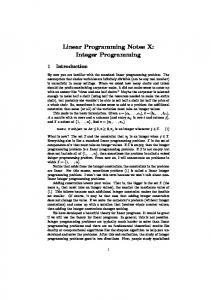
Example 1.1 Fig. 1 shows two arithmetic functions f0 = 3 ; 4x + 4xy + xz ; 2y + yz and
f1 = 4x0 + 2x1 + x2 represented in evbdds. The second function is derived as follows: f1 fx0 fx1 fx2
= 0 + fx0 = x0(4 + fx1 ) + (1 ; x0)fx1 = 4x0 + 2x1 + x2, = x1(2 + fx2 ) + (1 ; x1)fx2 = 2x1 + x2, = x2(1 + 0) + (1 ; x2)0 = x2.
2
Figure 1 goes here. A generic (evbdd) apply operator is described in �27]. This operator takes hcf � f i� hcg � gi and op as arguments and returns hch � hi such that ch + h � (cf + f ) op (cg + g) where op can be any operator which is closed over the integers. 3
evbdd representation enjoys a distinct feature, called the additive property, which is not seen in the obdd representation. For example, consider the following operation:
(cf + f ) ; (cg + g) = (cf ; cg ) + (f ; g). Because the values cf and cg can be separated from the functions f and g, the key for this entry in comp table is hh0� f i� h0� gi� ;i. After the computation of hh0� f i� h0� gi� ;i resulting in hch � hi, we then add cf ; cg to ch to have the complete result of hhcf � f i� hcg � gi� ;i. Hence, every operation hhc0f � f i� hc0g � gi� ;i can share the computation result of hh0� f i� h0� gi� ;i. This then will increase the hit ratio for caching the computation results. Another property of the evbdd representation, called the bounding property, is the following: when the maximum or minimum of a function exceeds a boundary value, then the result can be determined without further computation. As an example, the following pseudo code leq0(hcf � f i) performs operation (cf + f ) 0: leq 0(hcf � f i) f 1 if ((cf + max(f )) � 0) return(h1� 0i)� 2 if ((cf + min(f )) > 0) return(h0� 0i)� 3 if (comp table lookup(hcf � f i� leq 0� ans)) return(ans)� 4 hch � h i = leq 0(hcf + value(f )� childl(f )i)� 5 hch � h i = leq 0(hcf � childr(f )i)� 6 if (hch � h i == hch � h i) return (hch � h i)� 7 h = find or add(variable(f )� h � h � ch ; ch )� 8 comp table insert(hcf � f i� leq 0� hch � hi)� 9 return (hch � hi)� g l
l
r
r
l
l
r
r
l
l
l
r
r
l
r
r
A comp table storing previously computed results is used to achieve computation e�ciency. The entries of comp table are used in line 3 and stored in line 8. After the left and right children have been computed resulting in hch � h i and hch � h i (lines 4 and 5), if hch � h i = hch � h i, the algorithm returns hch � h i to ensure that the case of hx� k� k� 0i will not occur� otherwise, it returns hch � hvar, h , h � ch ; ch ii to preserve the property of right edge value being 0. There is another table (uniq table) used for the uniqueness property of evbdd nodes. Before leq0 returns its result, it checks this table through operation find or add which either adds a new node to the table or returns the node found in the table. To speed up the relational operators and the minimize (Sec. 2.3) operation, we include the minimum and maximum function values in each evbdd node. For the sake of readability, l
l
l
r
r
r
4
l
l
l
r
l
l
r
r
r
we also use the �attened evbdd as de ned below.
De�nition 1.3 A �attened evbdd is a directed acyclic graph consisting of two types of nodes. A nonterminal node v is represented by a 3-tuple hvariable(v)� childl(v)� childr(v)i where variable(v) 2 fx0� : : : � xn;1g. A terminal node v is associated with an integer v. Reduced, ordered, attened evbdds are de ned in the same way as obdds.
Example 1.2 The attened evbdd for the function in Fig. 1 (b) is shown in Fig. 2.
2
Figure 2 goes here. Multi-terminal binary decision diagram (mtbdd) which was recently proposed in �11] is the same as attened evbdd. In general, in functions where the number of distinct terminal values is large, mtbdd will require larger number of nodes than evbdd. However, in functions where the number of distinct terminal values is small, mtbdd may require less storage space depending on the number of nodes in the corresponding graphs. From Example 1.1 (Fig. 1(b)) and Example 1.2 (Fig. 2), we see that evbdd requires n + 1 nodes to represent 2n;1 x0 + : : : + 20xn;1 while attened evbdd (or mtbdd) require 2n+1 ; 1 to represent the same function. When there are only two di�erent terminal nodes (e.g., 0 and 1), evbdd, mtbdd, and obdd are equivalent in terms of the number of nodes and the topology of the graph �32]. In this case, evbdd will require more space to represent the the edge-values. The worst case time complexity for performing operations on evbdds is the same as that for mtbdds. However, due to the additive, bounding, and domain-reducing properties of evbdds, many operations on evbdds are much more e�cient the corresponding ones on mtbdds. Details can be found in �32].
The remainder of this paper is organized as follows. Three applications of evbdds: solving ilp problems, computing spectral coe�cients, and performing multiple output Boolean function decomposition are presented in sections 2, 3, and 4, respectively. Conclusions are given in section 5. 5
2 Integer Linear Programming Integer Linear Programming (ilp) is an np-hard problem �18] that appears in many applications. Most of existing techniques for solving ilp such as branch and bound �33, 13, 38] and cutting plane methods �19] are based on the linear programming (lp) method. While they may sometimes solve hundreds of variables, they cannot guarantee to nd an optimal solution for problems with more than , say, 50 variables. It is believed that an e�ective ilp solver should incorporate integer or combinatorial programming theory into the linear programming method �4]. Jeong et al. �25] describe an obdd-based approach for solving the 0-1 programming problems. This approach does not, however, use obdds for integer related operations such as conversion from linear inequality form of constraints into Boolean functions and optimization of nonbinary goal functions. Consequently, the caching of computation results is limited to only Boolean operations (i.e., for constraint conjunction). Our approach for solving the ilp is to combine bene ts of the evbdd data structure (in terms of subgraph sharing and caching of computation results) with the state-of-the-art ilp solving techniques. We have developed a minimization operator in evbdd which computes the optimal solution to a given goal function subject to a constraint function. In addition, the construction and conjunction of constraints in terms of evbdds are carried out in a divide and conquer manner in order to manage the space complexity.
2.1 Background An ilp problem can be formulated as follows: minimize subject to
Xn cixi� Xi n ai�j xi =1
i=1 xi
bj � 1 j m�
integer:
The rst equation is referred as the goal function and the second equation is referred as constraint functions. Throughout this section we will assume the problem to be solved is a minimization problem. A maximization problem can be converted to a minimization problem by changing the sign of coe�cients in the goal function. There are three classes of algorithms for solving ilp problems �45]. The rst class is 6
known as the branch and bound method �33, 13, 38]. This method usually starts with an optimum continuous lp solution which forms the rst node of a search tree. If the initial solution satis es the integer constraints, it is the optimum solution and the procedure is terminated. Otherwise, we split on variable x (with value x� from the initial solution) and create two new subproblems: one with the additional constraint x bx�c and the other with the additional constraint x � bx�c + 1. Each subproblem is then solved using the lp methods, e.g., the simplex method �14] or the interior point method �26]. A subproblem is pruned if there are no feasible solutions, the feasible solution is inferior to the best one found, or all variables satisfy the integer constraints. In the last case, the feasible solution becomes the new best solution. The problem is solved when all subproblems are processed. Most commercial programs use this approach �34]. The second class is known as the implicit enumeration technique which deals with 0-1 programming �2, 3, 44]. Initially, all variables are free. Then, a sequence of partial solutions is generated by successively �xing free variables, i.e., setting free variables to 0 or 1. A completion of a partial solution is a solution obtained by xing all free variables in the partial solution. The algorithm ends when all partial solutions are completions or are discarded. The procedure proceeds similar to the branch and bound except that it solves a subproblem using the logical tests instead of the lp. A logical test is carried out by inserting values corresponding to a given (partial or complete) solution in the constraints. A complete solution is feasible if it satis es all constraints. A partial solution is pruned if it cannot reach a feasible solution or could only produce an inferior feasible solution (compared to the current best solution). One advantage of this approach is that we can use partial order relations among variables to prune the solution space. For example, if it is established that x y, then portions of the solution space which correspond to x = 1 and y = 0 can be immediately pruned �7, 22]. In the early days, these two methods were considered to be sharply di�erent. The branch and bound method is based on solving a linear program at every node in the search space and uses a breadth rst strategy. The implicit enumeration method is based on logical tests requiring only additions and comparisons and employs a depth rst strategy. However, successively versions of both approaches have borrowed substantially from each other �3]. The two terms branch and bound and implicit enumeration are now used interchangeably. The third class is known as the cutting-plane method �19]. Here, the integer variable constraint is initially dropped and an optimum continuous variable solution is obtained. 7
The solution is then used to chop o� the solution space while ensuring that no feasible integer solutions are deleted. A new continuous solution is computed in the reduced solution space and the process is repeated until the continuous solution indeed becomes an integer solution. Due to the machine round-o� error, only the rst few cuts are e�ective in reducing the solution space �45].
2.2 A Model Algorithm In this section, we rst show a straightforward method to solve the ilp problem using evbdds. We then describe how to improve this method in this and the following sections.
Example 2.1 We illustrate how to solve the ilp problems using evbdds through a simple
example. For the sake of readability, we use attened evbdds. The following is a 0-1 ilp problem: minimize 3x + 4y , subject to 6x + 4y � 8, (1) 3x ; 2y � 1, (2) x� y 2 f0� 1g. We rst construct an evbdd for the goal as shown in Fig. 3 (a). We then construct the constraints. The left hand side of constraint (1) represented by an evbdd is shown in Fig. 3 (b). After the relational operator has been applied on constraint (1), the resulting evbdd is shown in Fig. 3 (c). Similarly, evbdds for constraint (2) are shown in Fig. 3 (d) and (e). The conjunction of two constraints, Fig. 3 (c) and (e), results in the evbdd in Fig. 3 (f) which represents the solution space of this problem. A feasible solution corresponds to a path from the root to 1. We then project the constraint function c onto the goal function g such that for a given input assignment X , if c(X ) = 1 (feasible) then p(X ) = g(X )� otherwise p(X ) = infeasible value. For minimization problems, the infeasible value is any value which is greater than the maximum of g, and for maximization problems, the infeasible value is any value which is smaller than the minimum of g. In our example, we use 8 as the infeasible value. Thus, in Fig. 3 (g), the two leftmost terminal values have been replaced by value 8. The last step in solving the above ilp problem is to nd the minimum in Fig. 3 (g) which is 0. 2
8
Figure 3 goes here. The above approach has three problems: 1. Converting a constraint from inequality form to a Boolean function may require exponential number of nodes� 2. Even if all constraints can be constructed without using excessive amounts of memory, conjoining them altogether at once may create too big an evbdd� and 3. The operator projection is useful when we want to nd all optimal solutions. However, in many situations, we are interested in nding any optimal solution. Thus, full construction of the nal evbdd (e.g., Fig. 3 (g)) is unnecessary. In the remainder of this section, we will show how to overcome the rst two problems by divide and conquer methods. In the next section, we will present an operator minimize which combines the bene ts of computation sharing and branch and bound techniques to compute any optimal solution. In our ilp solver, called fgilp, every constraint is converted to the form AX ; b 0. Thus, we only need one operator leq0 to perform the conversion. AX < b is converted to AX ; b + 1 0 (since all coe�cients are integer)� AX � b is converted to ;AX + b 0� and AX = b is converted to two constraints AX ; b 0 and ;AX + b 0. Initially, every constraint is an evbdd representing the left hand side of an inequality (i.e., AX ; b) which requires n nonterminal nodes for an n-variable function. fgilp provides users with an n supp parameter such that only if a constraint has less than n supp supporting (dependent) variables, then it will be converted to a Boolean function. fgilp allows users to set another parameter c size to control the size of evbdds. Only if constraints, in Boolean function form, are smaller in size than this parameter, they will be conjoined. The function performed by leq0 is the same as LI to BDD(I ) of �25] where I is some representation of w1x1 + : : : + wnxn � T . Our evbdd representation of a linear inequality is more e�cient than their representation, because leq0 can cache computation results as in all evbdd operations while LI to BDD cannot. This is very important because the e�ciency of obdd operations heavily depends on the extent by which this property is exploited. In �25], the authors suggest that it is not advisable to replace an equality by two inequalities because the cost of testing terminal cases (lines 1 and 2) are the same for equality and inequality 9
relations. Our experiments, however, show a completely di�erent result. Performing two inequalities followed by one conjunction (all in terms of evbdd operations) is much faster than carrying out one equality. We think that the di�erence is due to our computation caching capability. Parameters n supp and c size provide two advantages. First, they provide fgilp with a space-time tradeo� capability. The more memory fgilp has, the faster it runs. Second, combined with the branch and bound technique, some subproblems may be pruned before the conversion to the Boolean functions or the conjunction of constraints are carried out. When there is only one constraint and it is in Boolean form, then the problem is solved through minimize. Otherwise, the problem is divided into two subproblems and is solved recursively. Since both the goal and constraint functions are represented by evbdds. The new goal and constraint functions for the rst subproblem are the left children of the root nodes of the current goal and constraints. Similarly, the new goal and constraint functions for the second subproblem are the right children of the root nodes of the current goal and constraints. Our main algorithm, ilp min, employs a branch and bound technique. In addition to goal and constraint functions, n supp, and c size, there are two parameters which are used as bounding condition: Lower bound is either given by the user or computed through linear relaxation or Lagrangian relaxation methods� Upper bound represents the best feasible solution found so far. The initial value of the upper bound is the maximum of the goal function plus 1. If the maximum of goal function is less than the lower bound (LB) or the minimum of goal function is greater than or equal to the upper bound (UB), the problem is pruned. Furthermore, if there exists a constraint whose minimum feasible solution is greater than or equal to the current best solution (upper bound), then again the problem is pruned.
10
ilp min(goal� constr� LB� UB� n supp� c size) f 1 if (max(goal) < LB ) return� 2 if (min(goal) � UB ) return� 3 if (9c 2 constr : minimize(goal� c� UB ) == 0) return� 4 new constr = conjunction constr(constr� c size)� 5 if (new constr has only one element) f 6 minimize(goal� new constr� UB )� 7 g 8 else f 9 hhgoall� new constrl i� hgoal r� new constrr ii = divide problem(goal� new constr� n supp)� 10 ilp min(goall� new constrl � LB� UB� n supp� c size)� 11 ilp min(goalr� new constrr � LB� UB� n supp� c size)� 12 g g
Example 2.2 We want to solve the following problem: minimize ;4x + 5y + z + 2w, subject to 3x + 2y ; 4z ; w � 0, 2x + y + 3z ; 4w � 0, x� y� z� w 2 f0� 1g.
Figure 4 goes here.
1. The initial goal and constraint evbdds are shown in Fig. 4 (a). Suppose both parameters n supp and c size are set to 4. 2. Since the number of supporting variables in the constraint evbdds is not less than 4, we divide the problem into two subproblems: one with x = 1 (Fig. 4 (b)) and the other with x = 0 (Fig. 4 (c)). The nal solution is the minimum of solutions to these two subproblems. 3. Next, we want to solve the subproblem with x = 1. Since the number of supporting variables in constraint evbdds is smaller than n supp, we convert the constraint evbdds into Boolean functions by carrying out operation leq 0 (Fig. 4 (d)). 11
4. Since the size of constraint evbdds are not less than c size, we divide the problem into two subproblems: one with y = 1 (Fig. 4 (e)) and the other with y = 0 (Fig. 4 (f)). 5. Now, we want to solve the subproblem with y = 1. Since the size of both constraint evbdds are less than c size, we conjoin them together and then solve this subproblem using the minimize operator (Sec. 2.3). 6. The remaining subproblems are solved in the same way. Note that the solution found from a subproblem can be used as an upper bound for the subproblems which follow.
2
2.3 The Operator minimize This operator is another key distinction between our approach and the one in �25]. Operator minimize takes advantage of the additive and bounding properties of evbdds to achieve much more computation sharing and pruning of the search space. These properties lead to big savings in the memory requirement and run time of the ILP solver because of the way the computed table entries are stored and updated as explained below. Operator minimize is similar to the apply operator with one additional parameter b. Given a goal function g, a constraint function c, and an upper bound b, minimize returns 1 if it �nds a minimum feasible solution v < b of g subject to c� otherwise, minimize returns 0. If v is found, b is replaced by v� otherwise, b is unchanged. Note that when minimize returns 0, it does not imply that there are no feasible solutions with respect to g and c. This is because minimize only searches for feasible solutions that are smaller than b. Those feasible solutions which are greater than or equal to b are pruned because of the branch and bound procedure. The parameter b serves two purposes: it increases the hit ratio for computation caching and is a bounding condition for pruning the problem space. To achieve the �rst goal, an entry of the computed table used by minimize has the form hg� c� hb� vii where v is set to the minimum of g which satis�es c and is less than b. If there is no feasible solution (with respect to g and c) which is less than b, then v is set to b. The following pseudo code implements minimize. Lines 1-8 test for terminal conditions. In line 1, if the constraint function is the constant function 0, there is no feasible solution. In line 2, if the minimum of the goal function is greater than or equal to the current best solution, the whole process is pruned. If the goal function is a constant function, it must be 12
less than bound� otherwise, the test in line 2 would have been true. Thus, a new minimum is found in line 3. In line 6, if the constraint function is constant 1, then the minimum of the goal function is the new optimum. Again, this must be true, otherwise, the condition tested in line 2 would have been true. Lines 9-17 perform the table lookup operation. If the lookup succeeds, no further computation is required� otherwise, we traverse down the graph in lines 19-26 in the same way as apply. Since minimize satis�es the additive property, we subtract cg from bound to obtain a new local bound (local bound) in line 9. cg will be added back to bound in lines 13 or 32 if a new solution is found. Suppose we want to compute the minimum of g subject to c with current local upper bound local bound. We look up the computed table with key hg� ci. If an entry hg� c, hentry:bound� entry:valueii is found, then there are the following possibilities: 1. entry:value < entry:bound, i.e., a smaller value v was previously found with respect to g, c, and entry:bound (i.e., the minimization of g with respect to c has been solved and the result is entry:value). (a) If entry:value < local bound, then entry:value is the solution we wanted. (b) Otherwise, the best we can �nd under g and c is entry:value which is inferior to local bound, so we return with no success. 2. entry:bound = entry:value, i.e., there was no feasible solution with respect to g, c, and entry:bound (i.e., there is no stored result for the minimization of g with respect to c and entry:bound). (a) If local bound � entry:bound, then we cannot possibly �nd a solution better than entry:bound for g under c. Therefore, we return with no success. (b) Otherwise, no conclusion can be drawn and further computation is required. Although there is no better feasible solution than entry:bound, it does not imply that there will be no better solution than local bound. In cases 1.b and 2.a pruning takes place (also computation caching), in case 1.a, computation caching is a success, while in case 2.b both operations fail. Note that there is no need for updating an entry (of the computed table) except in case 2.b. In lines 25-30, the branch whose minimum value is smaller is traversed �rst since this increases chances for pruning the other branch. Finally, we update computed table and return the computed results in lines 31-39. 13
minimize(hcg� gi� hcc� ci� bound) f
/* test for terminal conditions */
8
hcc� ci == h0� 0i) return 0� if (min(hcg � gi) � bound) return 0� if (hcg � gi == hcg � 0i) f bound = cg � return 1� g if (hcc � ci == h1� 0i) f bound = min(hcg � gi)� return 1� g
9
local bound = bound ; cg �
1 2 3 4 5 6 7
if (
/* use the additive property */
/* look up the computed table */ 10 11 12 13 14 15 16 17 18
comp table lookup(h0� gi� hcc� ci� entry)) f entry:value < entry:bound) f if (entry:value < local bound) f bound = entry:value + cg � return 1� g else return 0� g else f if (local bound � entry:bound) return 0� g g entry:bound = local bound� if (
if (
/* create two subproblems by traversing down g and c */ 19 hcg � gli = hvalue(g)� childl(g)i� 20 hcg � gri = h0� childr(g)i� l
r
21 22 23
24
index(variable(c)) � index(variable(g))) f hcc � cli = hcc + value(c)� childl(c)i� hcc � cri = hcc� childr(c)i� g else f hcc � cli = hcc � cr i = hcc � ci� g
if (
l
r
l
r
/* solve the subproblem with lower minimum �rst */ 25 if (min(gl) � min(gr )) f 26 t ret = minimize(hcg � gli� hcc � cli� local bound)� 27 e ret = minimize(hcg � gri� hcc � cr i� local bound)� g l
28 29
30
r
r
r
f e ret = minimize(hcg � gri� hcc � cr i� local bound)� t ret = minimize(hcg � gli� hcc � cli� local bound)� g
else
l
/* a new minimum is found */ 31 32 33 34 35
37 38 39
g
l
t ret jj e ret) f bound = local bound + cg � entry:value = local bound� comp table insert(h0� gi� hcc� ci� entry )� return 1� g
if (
/* no new minimum is found */ 36
l
r
f entry:value = entry:bound� comp table insert(h0�14 gi� hcc� ci� entry )� return 0� g
else
Example 2.3 We want to minimize the goal function ;4x + 5y + z + 2w subject to the constraint (xzw� _ x�yzw� _ x�y�z _ x�y�z�w = 1) shown in Fig. 5. For the sake of readability, the
goal function is represented in evbdd while the constraint function is represented in obdd. The initial upper bound is max(goal) + 1 = 0 + 5 + 1 + 2 + 1 = 9. The reason for plus 1 is to recognize the case when there are no feasible solutions.
(a) We traverse down to nodes a and b through path x = 1 and y = 1. By subtracting the coe�cients of x and y from upper bound, we have 9 ; (;4) ; 5 = 8 which is the local upper bound with respect to nodes a and b. That is, we look for a minimum of a subject to b such that it is smaller than 8. It is easy to see that the best feasible solution of a subject to b is 1 which corresponds the assignments of z = 1 and w = 0. Thus, we insert ha� b� h8� 1ii as an entry into the computed table and recalculate the upper bound as ;4 + 5 + 1 + 0 = 2. (b) We traverse down to nodes a and b this time through path x = 1 and y = 0. The new local upper bound is 2 ; (;4) ; 0 = 6, i.e., we look for a feasible solution which
is smaller than 6. From computed table look up, we �nd that 1 is the best solution with respect to a and b and it is smaller than 6. Thus, the new upper bound is ;4 + 0 + 1 = ;3. (c) We reach a and b through path x = 0 and y = 1. The local upper bound is ;3 ; 0 ; 5 = ;8. Again, from the computed table, we know 1 is the best solution which is larger than ;8. Thus, no better solution can be found under a and b with respect to bound ;8 and the current best solution remains ;3. (d) We reach nodes a and c through path x = 0 and y = 0. The local upper bound is ;3 ; 0 ; 0 = ;3. The minimum of the goal function a is 0 which is greater than ;3. The optimal solution is ;3 with x = 1� y = 0� z = 1, and w = 0.
Figure 5 goes here.
15
2
2.4 Discussion A branch and bound/implicit enumeration based ilp solver can be characterized by the way it handles search strategies, branching rules, bounding procedures and logical tests. We will discuss these parameters in turn to analyze and explore possible improvements to fgilp. Search Strategy Search strategy refers to the selection of next node (subproblem) to process. There are two extreme search strategies. The �rst one is known as breadth �rst which always chooses nodes with best lower bound �rst. This approach tends to generate fewer nodes. The second one is depth �rst which chooses a best successor of the current node, if available, otherwise backtracks to the predecessor of the current node and continues the search. This strategy requires less storage space. fgilp uses the depth �rst strategy. Branching Rule This parameter refers to the selection of next variable to branch. Various selection criteria which have been proposed use priorities �37], penalties �15], pseudo-cost �5], and integer infeasibility �3] conditions. Currently, fgilp uses the same variable ordering as the one used to create evbdds because it simpli�es the implementation. When the variable selected does not correspond to the variable ordering of evbdd, operation cofactor (instead of childl and childr ) should be used. Bounding Procedure The most important component of a branch and bound method is the bounding procedure. The better the bound, the more pruning of the search space. The most frequently used bounding procedure is to use the linear programming method. Other procedures which can generate better bounds, but are more di�cult to implement include the cutting planes, Lagrangian relaxation �43], and disjunctive programming �4]. The bounding procedure used in fgilp is similar to the one proposed in �2]. In our experience, the most pruning takes place at line 3 of the code for ilp min. This pruning rule however has two weak points. First, it is carried out on each constraint one at a time. Thus, it is only a `local' method. Second, it can only be applied to a constraint which is in the Boolean form. The other bounding procedures described above are `global' methods which are directly applicable to the inequality form. Logical Tests It is believed that logical tests may be as important as the bounding procedure �39]. In addition to partial ordering of variables, a particularly useful class of tests, when available, 16
are those based on dominance �24, 25]. Currently, fgilp employs no logical tests. We believe that the inclusion of logical tests in fgilp will improve its performance. Despite the fact that there are many improvements which can be made to fgilp, the performance of our ilp solver, as it is now, is already comparable to that of lindo �42] which is one of the most widely used commercial tools �39] for solving ilp problems.
2.5 Experimental Results fgilp has been implemented in C under the sis environment. Table 1 shows our experimental results on ilp problems from miplib �36]. It also shows the results of lindo �42] (a commercial tool) on the same set of benchmarks. fgilp was run under sparc station 2 (28.5 mips) with 64 mb memory while lindo was run under sparc station 10 (101.6 mips) with 384 mb memory. In Table 1, column `Problem' lists the name of problems, columns `In-
puts' and `Constraints' indicate the number of input variables and constraints, and columns `fgilp' and `lindo' are the running time in seconds for obtaining the optimal solution shown in the last column. fgilp provides three options for the order in which constraints are conjoined together. When all constraints are conjoined together, the order of conjunction will not a�ect the size of �nal evbdd, but it does a�ect sizes of the intermediate evbdds. It is possible that an intermediate evbdd has size much larger than the the �nal one. Our motivation for this ordering is to control the required memory space and save computation time. These three options are: 1. Based on the order of constraints in the input �le. This provides users with direct control of the order. 2. evbdds with smallest size are conjoined �rst.
3. Constraints with the highest probability of not being satis�ed are conjoined �rst. The parameters used for the problems in Table 1 are summarized below: 1. Constraint conjunction order. Using the third option in problem `p0201' led to much less space and computation time than the other two options. The same option led to more time in other problems due to the overhead of computing the probability of function values being 0. For consistency, results are reported for this option only. 17
2. evbdd size of constraints. Without setting c size, `bm23' failed to �nish and `stein27' required 71.56 seconds. The run time reported in Table 1 for the above two problems were obtained by setting c size = 8000 while others were run under no limitation of c size. In general, this parameter has a signi�cant impact on the run time. We believe that the correct value for c size is dependent on the size of available memory for the machine. 3. Size of supporting variables. There was no limitation on the size of n supp. As results indicate, the performance of fgilp is comparable to that of lindo. Since ilp is an NP-complete problem, it is quite normal that one solver outperforms the other solver in some problems while performs poorly in others. Since sparc station 10 is about 5X faster than sparc station 2, fgilp runs faster than lindo on the examples reported above. lindo aborted on `bm23' with the following message: \Fatal out-of-space in invert, Re-installing best solution ..., Search aborted for numerical reasons". fgilp, however, requires much more space than lindo. As technology improves, memory is expected to become cheaper in cost and smaller in size. Increasing the available memory size will improve the speed of fgilp while will not bene�t lindo as much. The amount of space needed by fgilp is a function of not only the number of variables and constraints but also the structure of the constraint space in relation to the goal function. In some cases, fgilp handles problems with thousands of constraints, in other cases, it runs out of space in problems with a few hundred constraints.
Table 1 goes here.
3 Spectral Transformation The main purpose of spectral methods �47] is to transform Boolean functions from Boolean domain into another domain so that the transformed functions have more compact implementations. It was conjectured that these methods would provide a uni�ed approach to the 18
synthesis of analog and digital circuits �46]. Although spectral techniques have solid theoretical foundation, until recently they did not receive much attention due to their expensive computation times. With new applications in fault diagnosis, spectral techniques have recently invoked interest �23]. New computational methods have been proposed. In �17], a technique based on arrays of disjoint on- and dc-cubes is proposed. In �46], a cube-based algorithm for linear decomposition in spectral domain is proposed. Recently, �11] proposed two obdd-based methods for computing spectral coe�cients. The �rst method was to treat integers as bit vectors and integer operations as the corresponding Boolean operations. The main disadvantage of this representation is that arithmetic operations must be performed bit by bit which is very time consuming. The second method employed a variation of obdd called Multi-Terminal Binary Decision Diagrams (mtbdds) �10] which are exactly the same as the �attened form of evbdds. The major problem with using mtbdds is the space requirement when the number of distinct coe�cients is large. We propose evbdd-based algorithms for computing Hadamard (sometimes termed WalshHadamard) spectrum �47]. In our approach, the matrix representing Boolean function values used in spectral methods is represented by evbdds. This takes advantage of compact representation through subgraph sharing. The transformation matrix and the transformation itself are carried out through evbdd operations. Thus, the bene�t of caching computational results is achieved. In �11], the Walsh-Hadamard matrix and Boolean functions are represented by mtbdds and the spectral transformation is carried out by matrix operations on mtbdds. In our approach, no representation of this matrix is required as the transformation is carried out by addition and subtraction on evbdds. It remains to be seen that which implementation of the Walsh-Hadamard transformation is superior. As a footnote, if the number of distinct coe�cients of a function is large, it is more advantageous to use the evbdd implementation. However, due to the overhead of representing edge-values, for functions with small number of distinct coe�cients, the mtbdd implementation may be better. The reason we use the Hadamard transformation rather than other transformations (e.g., Walsh, Rademacher-Walsh, and Walsh-Paley �23]) is that the Hadamard transformation matrix has the recursive Kronecker product structure which perfectly matches the recursive structure of evbdds. The algorithms presented here include both the transformation from Boolean domain to spectral domain and the operations within the spectral domain itself. 19
The Hadamard transformation is carried out in the following form:
T n Z n = Rn �
(1)
where T n is a 2n � 2n matrix called transformation matrix, Z n is a 2n � 1 matrix which is the truth table representation ofa Boolean function, Rn is a 2n � 1 matrix which is the spectral coe�cients of a Boolean function. Di�erent transformation matrices generate di�erent spectra. Here, we use the Hadamard transformation matrix �47] which has a recursive structure as follows:
Tn
=
"
#
T n;1 T n;1 � T n;1 ;T n;1
T 0 = 1:
Example 3.1 The spectrum of function f (x� y) = x � y is computed as 2
32
1 1 1 1 76 0 6 6 1 ;1 1 ;1 77 66 1 6 6 1 1 ;1 ;1 75 64 1 4 1 ;1 ;1 1 0
3 7 7 7 7 5
2
3
27 6 6 0 7 = 66 0 77 : 4 5 ;2
The order of each spectral coe�cient ri (ith row of Rn ) is the number of 1's in the binary representation of i� 0 � i � 2n ; 1. For example, r00 is the zeroth-order coe�cient, r01 and r10 are the �rst-order coe�cients, and r11 is the second-order coe�cient. Let Rni = f multi-set of the absolute value of rk 's where rk is an ith-order coe�cient of Rn g, 0 � i � n. In Example 3.1, R20 = f2g, R21 = f0� 0g, and R22 = f2g. An operation on f and its Rn which does not modify the sets Rni is referred as an invariance operation. Given a function f (x1� : : :� xn) with spectrum Rn , three invariance operations on f and Rn are as follows (formal proofs may be found in �16]): 1. Input negation invariance: if xi is negated, then the new spectrum Rn is formed by rk0 = ;rk where the ith bit of k is 1, and rk0 = rk otherwise. 0
2. Input permutation invariance: if input variables xi and xj are exchanged, then the new spectrum is formed by exchanging rk 's and rl's where k ; 2i = l ; 2j . That is, the ith and j th bits of k and l are h1� 0i and h0� 1i, respectively, while all other bits of k and l are the same. 20
3. Output negation invariance: if f is negated, the Rn is formed by replacing all rk by ;rk . 0
Lemma 3.1 Two Boolean functions are input-negation, input-permutation, and outputnegation equivalent (npn-equivalent) only if their Rni 's are equivalent.
With this property, Rni can be used as a �lter to improve performance in a Boolean matching algorithm as presented in �28].
3.1 Spectral evbdd (spbdd) The major problem with Equation 1 is that all matrices involved are of size 2n . Therefore, only functions with a small number of inputs can be computed. We overcome this di�culty by using evbdds to represent both Z n and Rn . When an evbdd is used to represent Rn , we refer to it as SPectral evbdd, or spbdd for short. The di�erence between evbdds and spbdds is in the semantics, not the syntax. A path in evbdds corresponds to a function value while a path in spbdds corresponds to a spectral coe�cient. The matrix multiplication by T n is implicitly carried out in the transformation from Z n to Rn (i.e., from evbdd to spbdd). We de�ne Z n and Rn recursively as follows: " n;1 # n Z = ZZ0n;1 � 1
Rn
=
"
#
Rn0 ;1 : Rn1 ;1
Then, Equation 1 can be rewritten as: " n;1 n;1 # " # T Z0 + T n;1Z1n;1 = Rn0 ;1 : T n;1Z0n;1 ; T n;1Z1n;1 Rn1 ;1 Equation 2 then is implemented through evbdd 1 as :
� (hx� Z1n;1� Z0n;1 i) = hx� � (Z0n;1) ; � (Z1n;1)� � (Z0n;1) + � (Z1n;1 )i� � (1) = 1� � (0) = 0: 1 For
the sake of readability, we use �attened
evbdd in this section.
21
(2) (3)
where � is the transformation function which converts an evbdd representing a Boolean function to an spbdd. To show the above equations correctly implement Equation 2, we prove the following lemma.
Lemma 3.2 Let � : evbdd ! spbdd as de�ned in Equations 3-4, then � implements T , that is, � (f n ) = T nf n , where f n is an n-input function. Or, equivalently, � (hxn� Z1n;1� Z0n;1 i) = hxn � Rn1 ;1 � Rn0 ;1i. Example 3.2 The exclusive-or function in Example 3.1 is redone in terms of evbdd representation. � (hx� hy� 0� 1i� hy� 1� 0ii) = hx� � (hy� 1� 0i) ; � (hy� 0� 1i)� � (hy� 1� 0i) + � (hy� 0� 1i)i = hx� hy� ;1� 1i ; hy� 1� 1i� hy� ;1� 1i + hy� 1� 1ii = hx� hy� ;2� 0i� hy� 0� 2ii
Pseudo code evbdd to spbdd(ev� level� n) is the implementation of Equation 2. Because of the following situation, this procedure requires level and n as parameters: � (hx� z� zi) = hx� � (z) ; � (z)� � (z ) + � (z)i, = hx� 0� 2 � � (z )i: In reduced evbdd, hx� z� zi will be reduced to z while hx� 0� 2 � � (z)i cannot be reduced in spbdd. We need to keep track of the current level so that when the index of the root node ev is greater than level, we generate hlevel� 0� 2 � � (ev)i (lines 3-8). evbdd to spbdd(ev� level� n) f 1 if (level == n) return ev � 2 if (ev == 0) return 0� 3 if (index(ev ) > level) f 4 sp = evbdd to spbdd(ev� level + 1� n)� 5 left = 0� 6 right = evbdd add(sp� sp) 7 return new evbdd(level� left� right)� 8 g 9 spl = evbdd to spbdd(childl(ev)� level + 1� n)� 10 spr = evbdd to spbdd(childr(ev)� level + 1� n)� 11 left = evbdd sub(spr � spl )� 12 right = evbdd add(spr � spl)� 13 return new evbdd(level� left� right)� g
22
3.2 Boolean Operations in Spectral Domain In this section, we show how to perform Boolean operations in spbdds. We �rst present the algorithm for performing Boolean conjunction in spbdds by the following de�nition.
De nition 3.1 Given two spbdds f and g, the operator ^ is carried out in the following way. If f and g are terminal nodes, then
f ^ g = f � g: Otherwise,
hx� fl� fr i ^ hx� gl� gr i = hx� (fl ^ gr + fr ^ gl )=2� (fl ^ gl + fr ^ gr )=2i:
The following lemma and theorem prove that the above de�nition carries out the Boolean conjunction in spbdds.
Lemma 3.3 (f + g) ^ (i + j ) = f ^ i + f ^ j + g ^ i + g ^ j , where f� g� i� j 2 spbdd. (Note that +'s may be replaced by ;'s.) Theorem 3.1 Given two Boolean functions f and g represented in evbdds, � (f g) = � (f ) ^ � (g), where is the conjunction operator in Boolean domain. Other Boolean operations in spbdds are carried out by the following equations:
f _ g = f + g ; f ^ g� f � g = f + g ; 2 � (f ^ g)� f� = J n ; f�
(4) (5) (6)
where = _� �� and �� are or, xor, and not in spectral domain (spbdd), J n = �2n� 0� : : : � 0]t. These operations _� �, and�are from �23] with minor modi�cation to match the � operation. Operations +� ;, and � are carried out in the same way as in evbdds (e.g., apply in �27]).
23
3.3 Experimental Results Table 2 shows the results of some benchmarks represented in both evbdd and spbdd forms. Column `evbdd' depicts the size and time required for representing and constructing a circuit using evbdds while column `spbdd' depicts the size of spbdds and the time required for converting from evbdds to spbdds. In average, the ratio of the number of nodes required for representing spbdds over that of evbdds is 6.8, and the ratio of the conversion time for spbdds over the construction time of evbdds is 41. One application of spectral coe�cients is that they can be used as a �lter for pruning search space in the process of Boolean matching �11, 28]. The performance of a �lter depends on its capability of pruning (e�ectiveness) and its computation time (cost). Experimental results of �11] show that this �lter is quite good because this �lter rejected all unmatchable functions that were encountered. However, according to results of Table 2, this �lter is relatively expensive to compute when comparing with other �lters �28]. We believe that this �lter should be used only after other �lters have failed to prune.
Table 2 goes here.
4 Function Decomposition While a problem with �nite domain can be solved by conversion to Boolean functions, a problem related to multiple-output Boolean functions can also be solved by interpreting them as the bit representation of an integer function. For example, a multiple-output Boolean function hf0� : : : � fm;1i can be transformed to an integer function F by F = 2m;1 f0 + : : : + 20fm;1 . Based on this formulation, we present the application of evbdds to performing function decomposition of multiple-output Boolean functions. The motivation for using function decomposition in logic synthesis is to reduce the complexity of the problem by a divide-and-conquer paradigm: A function is decomposed into a set of smaller functions such that each of them is easier to synthesize. The function decomposition theory was studied by Ashenhurst �1], Curtis �12], and Roth and Karp �40]. In Ashenhurst-Curtis method, functions are represented by Karnaugh maps 24
and the decomposability of functions are determined from the number of distinct columns in the map. In Roth-Karp method, functions are represented by cubes and the decomposability of functions are determined from the cardinality of compatible classes. Recently, researchers �6, 9, 29, 41] have used obdds to determine decomposability of functions. However, most of these works only consider single-output Boolean functions. In this section, we start with de�nitions of function decomposition and cut sets in evbdd representation. Based on the concept of cut sets, we develop an evbdd-based disjunctive decomposition algorithm.
4.1 De nitions De nition 4.1 A pseudo Boolean function f (x0� : : : � xn;1) is said to be decomposable under bound set fx0� : : :� xi;1 g and free set fxi � : : :xn;1 g, 0 < i < n, if f can be transformed to f 0(g0(x0� : : : � xi;1)� : : :� gj (x0� : : :� xi;1)� xi� : : :� xn;1) such that the number of inputs to f 0 is smaller than that of f . If j equals 1, then it is simple decomposable.
Note that since inputs to a pseudo Boolean function are Boolean variables, function gk 's are Boolean functions. Here, we consider only disjunctive decomposition (the intersection of bound set and free set is empty).
De nition 4.2 Given an evbdd hc� vi representing f (x0� : : : � xn;1) with variable ordering x0 < : : : < xn;1 and bound set B = fx0� : : : � xig, we de�ne cut set(hc� vi� B ) = fhc0� v0i j hc0� v0i = eval(hc� vi� j )� 0 � j < 2i g. For the sake of readability, we use the �attened form of evbdds in this section.
Example 4.1 Given a function f as shown in Fig. 6 with bound set B = fx0� x1� x2g, cut set(f� B ) = fa� b� c� dg. 2 Figure 6 goes here. If an evbdd is used to represent a Boolean function, then each node in the cut set corresponds to a distinct column in the Ashenhurst-Curtis method �1, 12] and a compatible class in the Roth-Karp decomposition algorithm �40]. 25
4.2 Disjunctive Decomposition �9, 29, 41] describe algorithms for disjunctive decomposition of single-output Boolean functions based on the obdd representation of these functions. However the concept of communication links used in �9, 41] cannot be directly applied to multiple output functions. Here, we present an evbdd-based disjunctive decomposition algorithm which is an extension of the algorithm presented in �29]. Algorithm D: Given a function f represented in an evbdd vf and a bound set B , a disjunctive decomposition with respect to B is carried out in the following steps: 1. Compute the cut set with respect to B . Let cut set(v� B ) = fu0� : : : � uk;1 g. 2. Encode each node in the cut set by dlog2 ke = j bits. 3. Construct vm's to represent gm 's, 0 � m < j : Replace each node u with encoding b0� : : : � bj;1 in the cut set by terminal node bm. 4. Construct vf to represent function f 0: Replace the top part of vf by a new top on variables g0� : : : � gj;1 such that eval(vf � l) = ul for 0 � l < k ; 1, eval(vf � l) = uk;1 for k ; 1 � l < 2j . 0
0
0
The correctness of this algorithm can be intuitively argued as follows: For any input pattern m in the bound set, the evaluation of m in function f will result at a node in the cut set with encoding e. The evaluation of m on the gl functions should thus produce the function values e. The evaluation of e in function f 0 should also end at the same node in the cut set. Thus, the composition of f 0 and gl's becomes equivalent to f . In step 2 of Algorithm D, we use an arbitrary input encoding which is not unique. Di�erent encodings will result in di�erent decompositions. Furthermore, when k < 2j , not every j -bit pattern is used in the encoding of the cut set� Function gl 's can never generate function values which correspond to the patterns absent from the encoding, thus we can assign these patterns to any node in the cut set. In step 4, we assign them to the last node in the cut set (uk;1 ). Alternatively, we could have made them into explicit don't-cares.
Lemma 4.1 Given an
evbdd vf with variable ordering x0 < : : : < xn;1 representing f (x0� : : :� xn;1), a bound set B = fx0� : : :� xi;1g and cut set(vf � B ) = fu0� : : :� uk;1 g, if Algorithm D returns evbdds vf � vg0 � : : : � vgj 1 , then 0
;
f (x0� : : : � xn;1) = f 0(g0(x0� : : :� xi;1)� : : :� gj;1 (x0� : : : � xi;1)� xi� : : : � xn;1) where f 0� g0� : : :� gj;1 are the functions denoted by vf � vg0 � : : :� vgj 1 , respectively. 0
26
;
Example 4.2 Fig. 7 shows an example of disjunctive decomposition in evbdds. The eval-
uation of the input pattern x0 = 1, x1 = 0, and x2 = 1 in function F will end at the leftmost x4-node which has encoding 10. The evaluation of the same input pattern in functions g0 and g1 would produce function values 1 and 0. Then, with g0 being 1 and g1 being 0 in function F 0, it would also end at the leftmost x4-node. 2
Figure 7 goes here. When an evbdd is used to represent a Boolean function, Algorithm D corresponds to a disjunctive decomposition algorithm for Boolean functions� when an evbdd represents an integer function, then Algorithm D can be used as a disjunctive decomposition algorithm for multiple-output Boolean functions as shown in the following example.
Example 4.3 A 3-output Boolean function as shown in Fig 8 (a) can be converted into
an integer function as shown in Fig. 8 (b) through F = 4f0 + 2f1 + f2. The application of Algorithm D on F is the one shown in the previous example. After decomposition, we can 2 convert F 0 back to a 3-output Boolean function f00 , f10 , and f20 .
Figure 8 goes here.
4.3 Computing Cut sets for All Possible Bound Sets In the previous section, we showed how to perform function decomposition directly on evbdds when a bound set is given. In this section, we show how to compute the cut sets for all bound sets of (single-output) Boolean functions. Our method is based on the encoding of columns of the decomposition chart where free variables de�ne the rows and bound variables de�ne the columns �1, 12]. Decomposability is determined by the number of distinct columns (i.e., bit vectors). By encoding these bit 27
vectors as integers, we transform the problem to that of computing the cardinality of a set of integers. Initially, every variable is in the free set. For each variable xi, we perform the following two operations: 1. include: include xi in the bound set to derive a new cut set, and 2. exclude: partially encode the columns such that distinct columns are given unique codes and variable xi is permanently excluded from the bound set.
Example 4.4 Fig. 9 (a) shows a decomposition chart where variable x is in the free set
and a� b� c� d� e� f� and g are Boolean values. To perform the include operation, we move the bottom two rows to the left of the top two rows such that x now is in the bound set (Fig. 9 (b)). To perform the exclude operation, we encode bit vectors hc� ai, hd� bi, hg� ei, and hh� f i as 2c + a, 2d + b, 2g + e, and 2h + f , respectively (Fig. 9 (c)). The coded decomposition chart preserves the distinctness of columns, that is, column ha� b� c� di is distinct from column he� f� g� hi if and only if column h2c + a� 2d + bi is distinct from column h2g + e� 2h + f i. Furthermore, variable x is absent from the encoded decomposition chart and will never be included in the bound set. 2
Figure 9 goes here. Given an evbdd v with the top variable xi, the right and left children of v correspond to the top and bottom halves of rows in the decomposition chart. Thus, operations include and exclude in the evbdd representation are carried out in the following way: 1. include: construct the set fchildl(v)� childr(v)g, and 2. exclude: construct an evbdd representing 22 � childl(v) + childr (v) where 22 is to ensure that the resulting evbdd has a unique encoded representation. i
i
Example 4.5 Fig. 10 (a) is the evbdd representation of the decomposition chart in Fig. 9
(a). The corresponding operations include and exclude are shown in Fig. 10 (b) and (c), respectively. 2 28
Figure 10 goes here. Pseudo code cut set all computes the cardinality of the cut set for every possible bound set of a given function. The routine returns the set fhb� ki j b is a bound set and k is the cardinality of the cut set of bg. Initially, we have i = 0 and node set = fvg where v is the evbdd representing the given function. This corresponds to the bound set B = � and free set X where X is the set of input variables. If i = n, then we reach the terminal case and node set is the (encoded) cut set for bound set B (line 1)� otherwise, we perform include and exclude operations with respect to variable xi (lines 2 and 3). We repeat the process for variable xi+1 in lines 4 and 5. In line 6, the union of hb� ki's from lines 4 and 5 is returned. Pseudo code include and exclude perform the include and exclude operations for a set of evbdd nodes. cut set all(node set� B� i) f 1 if (i == n) return(fhB� j node set jig)� 2 inc set = include(node set� i)� 3 exc set = exclude(node set� i)� 4 inc = cut set all(inc set� B � fxig� i + 1)� 5 exc = cut set all(exc set� B� i + 1)� 6 return(inc � exc)� g include(node set� i) f 1 new set = �� 2
if (
4 5 6
u 2 node set f index(variable(u)) == i) new set = new set � fchildl(u)� childr(u)g� else = � index(u) > i � = new set = new set � fug�
for each node
3
7
g
8
return
g
new set�
29
exclude(node set� i) f 1 new set = �� 2 3
if
4 5 6
u 2 node set f (index(variable(u)) == i)
for each node
new set = new set � f22 � childl(u) + childr (u)g� else = � index(u) > i � = new set = new set � f22 � u + ug� i
7
g
8
return
g
i
new set�
Example 4.6 Fig. 11 (a) shows a function represented by both a truth table and a �attened
evbdd. Initially, the bound set is empty. The applications of include and exclude with
respect to variable x0 are shown in Fig. 11 (b) and (c), respectively. In Fig. 11 (b), the bound set is fx0g and the cardinality of the cut set is 2� In Fig. 11 (c), the bound set is � with cut set size 1. The application of include and exclude on Fig. 11 (b) with respect to variable x1 results in Fig. 12 (a) and (b) with bound sets fx0� x1g and fx0g and cut set sizes 2 and 2, respectively. The application of include and exclude on Fig. 11 (c) with respect to variable x1 results in Fig. 12 (c) and (d) with bound sets fx1g and � and cut set sizes 2 and 1, respectively. The application of include and exclude on Fig. 12 (b) with respect to variable x2 results in Fig. 13 (a) and (b) with bound sets fx0� x2g and fx0g and encoded cut sets f0� 1� 5� 4g and 5, 12, respectively. In Fig. 13, the top row shows the encoded decomposition charts, the second row shows the encoded cut sets, and the third row shows the decomposition charts. The encodings used for the bottom row in Fig. 13 (a) and (b) are 1 � row1 + 4 � row2 and 1 � row1 + 2 � row2 + 4 � row3 + 8 � row4, respectively. 2
Figure 11 goes here. Figure 12 goes here.
30
Figure 13 goes here. Since there are 2n di�erent bound sets for an n variable function, the computation of the cut set for every bound set is very expensive. If we replace line 1 in cut set all by 1 if (level == n jj j var set j� k) return(fhB� j node set jig), then cut set all becomes a routine for computing the cardinality of the cut set for every bound set whose size is less than or equal to k which is useful for the technology mapping of k-input look-up table �eld programmable gate arrays �31]. A naive way to compute the cut set for every bound set is to move the bound variables to the top of the evbdd. Compared to this approach, our approach has the following advantages. Firstly, it is well known that the size of obdd (and evbdd) is very sensitive to the variable ordering (at least in many practical applications �35]). Moving the bound variables to the top will change the variable ordering and hence may cause storage problems. Our method will not change the variable ordering. Secondly, the number of variables in the direct variable exchange approach is never reduced. In contrast, in our approach, after the include and exclude operations, the number of variables will be decreased by 1.
4.4 Experimental Results In order to evaluate the e�ectiveness of cut set all, we compared our program with the Roth-Karp decomposition algorithm implemented in sis. In particular, we used the following command on a number of mcnc91 benchmark sets: \xl k decomp2 -n 4 -e -d -f 100" which for every node in the Boolean network, �nds the best bound set of size � 4 that reduces the node's variable support after decomposition, and then decomposes the node, and modi�es the network to re�ect the change. We provided equivalent evbdd-based implementation of this sis command. To assign a unique encoding for each evbdd node, we need integers with 2i bits where i is the number of variables considered so far. This is clearly very expensive. One way to overcome this di�culty is to relax the uniqueness condition (e.g, use 2 instead of 22 ). Then, two di�erent evbdd nodes representing di�erent functions may be assigned the same encoding. As a result, the size of the cut set for a given bound set may be underestimated. i
2
xl k decomp
does not process circuits with
32 inputs.
31
This scheme may be used as a �lter. For example, to �nd the bound set which has the smallest cut set, we �rst perform cut set all to �nd the best ones, and then check for the real cut sets by moving the bound variables to the top of the evbdd. Results shown in Table 3 used 2 as the weight in exclude operation. We stopped the processes which took more that 5000 cpu seconds on a Sun Sparc-Station II with 64 MB of memory. We obtain signi�cant speed-ups (by an average factor of 35.4). Table 3 goes here.
5
Conclusions
Because of the compactness and canonical properties, obdds and evbdds have been shown e�ective for handling veri�cation problems �8, 27]� because of the additive property, evbdds are also useful for solving integer linear programming problems (e.g., Sec. 2). Boolean values are a subdomain of integer values and Boolean operations are special cases of arithmetic operations. With this interpretation, evbdds are particularly useful for applications which require both Boolean and integer operations. Examples are shown in performing spectral transformations (e.g., Sec. 3) and representing multiple output Boolean functions (e.g., Sec. 4). evbdds could be used for other applications. For example, �10] uses mtbdds to represent general matrices and to perform matrix operation such as standard and Strassen matrix multiplication, and lu factorization� �20] uses obdds to implement a symbolic algorithm for maximum �ow in 0-1 network. Equivalent evbdd-based algorithms can be developed to solve these problems.
References 1] R. L. Ashenhurst, \The decomposition of switching functions," Ann. Computation Lab., Harvard University, vol. 29, pp. 74-116, 1959. 2] E. Balas, \An additive algorithm for solving linear programs with zero-one variables," Operations Research, 13 (4), pp. 517-546, 1965.
32
3] E. Balas, \Bivalent programming by implicit enumeration," Encyclopedia of Computer Science and Technology Vol.2, J. Belzer, A.G. Holzman and Kent, eds., M. Dekker, New York, pp. 479494, 1975. 4] E. Balas, \Disjunctive programming," Annals of Discrete Mathematics 5, North-Holland, pp. 3-51, 1979. 5] M. Benichou, J. M. Gauthier, P. Girodet, G. Hentges, G. Ribiere and O. Vincent, \Experiments in mixed-integer linear programming," Math. Programming 1, pp. 76-94, 1971. 6] M. Beardslee, B. Lin, and A. Sangiovanni-Vincentelli, \Communication based logic partitioning," Proc. of the European Design Automation Conf., pp. 32-37, 1992. 7] V. J. Bowman, Jr. and J. H. Starr, \Partial orderings in implicit enumeration," Annals of Discrete Mathematics, 1, North-Holland, pp. 99-116, 1977. 8] R. E. Bryant, \Graph-based algorithms for Boolean function manipulation," IEEE Transactions on Computers, C-35(8): 677-691, August 1986. 9] S-C. Chang and M. Marek-Sadowska, \Technology mapping via transformations of function graph," Proc. International Conf. on Computer Design, pp. 159-162, 1992. 10] E. M. Clarke, M. Fujita, P. C. McGeer, K. L. McMillan, and J. C.-Y. Yang, \Multi-terminal binary decision diagrams: An e�cient data structure for matrix representation," International Workshop on Logic Synthesis, pp. 6a:1-15, May 1993. 11] E. M. Clarke, K. L. McMillan, X. Zhao, M. Fujita, and J. C.-Y. Yang, \Spectral transforms for large Boolean functions with applications to technology mapping," Proc. of the 30th Design Automation Conference, pp. 54-60, 1993. 12] H. A. Curtis, \A new approach to the design of switching circuits," Princeton, N.J., Van Nostrand, 1962. 13] R. J. Dakin, \A tree-search algorithm for mixed integer programming problems," Comput. J. 9, pp. 250-255, 1965. 14] G. B. Dantzig, Linear Programming and Extensions, Princeton, N. J.: Princeton University Press, 1963. 15] N. J. Driebeck, \An algorithm of the solution of mixed integer programming problems," Management Science 12, pp. 576-587, 1966. 16] C. R. Edwards, \The application of the Rademacher-Walsh transform to Boolean function classi�cation and threshold-logic synthesis," IEEE Transactions on Computers, C-24, pp. 4862, 1975. 17] B. J. Falkowski, I. Schafer and M. A. Perkowski, \E�ective computer methods for the calculation of Rademacher-Walsh spectrum for completely and incompletely speci�ed Boolean functions," IEEE Transaction on Computer-Aided Design, Vol. 11, No. 10, pp. 1207-1226, Oct. 1992.
33
18] M. R. Garey and D. S. Johnson, \Computers and Intractability: A Guide to the Theory of NP-Completeness," Freeman, San Francisco, 1979. 19] R. E. Gomory, \Solving linear programming problems in integers," in Combinatorial Analysis, R.E. Bellman and M. Hall, Jr., eds., American Mathematical Society, pp. 211-216, 1960. 20] G. D. Hachtel and F. Somenzi, \A symbolic algorithm for maximum �ow in 0-1 networks," International Workshop on Logic Synthesis, pp. 6b:1-6, May 1993. 21] P. L. Hammer and S. Rudeanu, Boolean Methods in Operations Research and Related Areas, Heidelberg, Springer Verlag, 1968. 22] P. L. Hammer and B. Simeone, \Order relations of variables in 0-1 programming," Annals of Discrete Mathematics, 31, North-Holland, pp. 83-112, 1987. 23] S. L. Hurst, D. M. Miller and J. C. Muzio, Spectral Techniques in Digital Logic, London, U.K. : Academic, 1985. 24] T. Ibaraki, \The power of dominance relations in branch and bound algorithm," J. Assoc. Comput. Mach. 24, pp. 264-279, 1977. 25] S-W. Jeong and F. Somenzi, \A new algorithm for 0-1 programming based on binary decision diagrams," Logic Synthesis Workshop, in Japan, pp. 177-184, 1992. 26] N. Karmarkar, \A new polynomial-time algorithm for linear programming," Combinatorica, 4:373-395, 1984. 27] Y-T. Lai and S. Sastry, \Edge-Valued binary decision diagrams for multi-level hierarchical veri�cation," Proc. of 29th Design Automation Conf., pp. 608-613, 1992. 28] Y-T. Lai, S. Sastry and M. Pedram, \Boolean matching using binary decision diagrams with applications to logic synthesis and veri�cation," Proc. International Conf. on Computer Design, pp.452-458, 1992. 29] Y-T. Lai, M. Pedram and S. Sastry, \BDD based decomposition of logic functions with application to FPGA synthesis," Proc. of 30th Design Automation Conf, pp. 642-647, 1993. 30] Y-T. Lai, M. Pedram and S. Vrudhula, \Edge-Valued Binary-Decision Diagrams: Theory and Applications," Technical Report 93-31, University of Southern California, Aug. 1993. 31] Y-T. Lai, K-R. Pan, M. Pedram, and S. Vrudhula, \FGMap: A Technology Mapping Algorithm for Look-Up Table Type FPGAs based on Function Graphs", International Workshop on Logic Synthesis, 1993. 32] Y-T. Lai, \Logic Veri�cation and Synthesis using Function Graphs," PhD Dissertation, Computer Engineering, Univ. of Southern Calif., December 1993. 33] A. H. Land and A. G. Doig, \An automatic method for solving discrete programming problems," Econometrica 28, pp. 497-520, 1960. 34] A. Land and S. Powell, \Computer codes for problems of integer programming," Annals of Discrete Mathematics 5, North-Holland, pp. 221-269, 1979.
34
35] H-T. Liaw and C-S Lin, \On the OBDD-representation of general Boolean functions," IEEE Trans. on Computers, C-41(6): 661-664, June 1992. 36] Department of Mathematical Sciences, Rice University, Houston, TX 77251. 37] G. Mitra, \Investigation of some branch and bound strategies for the solution of mixed integer linear programs," Math. Programming 4, pp. 155-170, 1973. 38] L. G. Mitten, \Branch-and-bound methods: General formulation and properties," Operations Research, 18, pp. 24-34, 1970. 39] G. L. Nemhauser and L. A. Wolsey, Integer and Combinatorial Optimization, Wiley, New York, 1988. 40] J. P. Roth and R. M. Karp, \Minimization over Boolean graphs," IBM Journal, pp. 227-238, April 1962. 41] T. Sasao, \FPGA design by generalized functional decomposition," in Logic Synthesis and Optimization, Sasao ed., Kluwer Academic Publisher, pp. 233-258, 1993. 42] L. Schrage, Linear, Integer and Quadratic Programming with LINDO, Scienti�c Press, 1986. 43] J. F. Shapiro, \A survey of lagrangian techniques for discrete optimization," Annals of Discrete Mathematics 5, North-Holland, pp. 113-138, 1979. 44] K. Spielberg, \Enumerative methods in integer programming," Annals of Discrete Mathematics 5, North-Holland, pp. 139-183, 1979. 45] H. A. Taha, \Integer programming," in Mathematical Programming for Operations Researchers and Computer Scientists, ed. A.G. Holzman, Marcel Derrer, pp.41-69, 1981. 46] D. Varma and E. A. Trachtenberg, \Design automation tools for e�cient implementation of logic functions by decomposition," IEEE Transactions of Computer-Aided Design, Vol. 8, No. 8, Aug. 1989, pp. 901-916. 47] J. S. Wallis, \Hadamard matrices," Lecture Notes No. 292, Springer-Verlag, New York, 1972.
35
0
3
x0
x -4
4
y 2
-2
z
z
2
x1
y 2
x2 1
1
0
0
(b)
(a)
Figure 1: Two examples.
36
x
0
x
x1
1
x2 7
6
x
5
x
x2
2
2
3
4
2
1
0
Figure 2: An example of �attened evbdd.
37
x y
y
3
7
4
y
0
x y
3 -2
0
0
4
x
x y
(d)
y 1
(e)
0
1
1 1
0
(c)
0 1
1
y
(b)
y
y
y
y
6
10
(a)
1
x
x
y
0 1
1
(f)
x y
8
y
8 4
0
(g)
Figure 3: A simple example (using �attened evbdds and obdds).
38
0
0
0
x
x
x
-4
3
2
y
1
2
5 z
z
z
1 w
w
w
0
0
0
3
w
-4
0
0
0 (c)
(b)
(a)
w
w -1
0
0
0
z
z -4
2
-4
-1
2
z
w
w
w
-4
-1
2
1
2
1
3
-4
1
y
y
5 z
z
z
3
-4
1
2
5
0
0
y
y
y
y
0
2
3
-4 y
y
-4 y
y
y
-4
1
5 z
z
z
z
z
z
1
1
1 w
1
w
0
w
w
0
w
w
w
0
1
0 (d)
1
0
1
0
0
w
2
2
2
z
z
z
z
z
0
1
0
1
0
(e)
Figure 4: An example for conjoining constraints.
39
1
0 (f)
0
0 x
x -4
y
y 5 z
z
b z
a
c
1 w
w
0
w
1
2 0
0
1
1
0
(b)
(a)
Figure 5: An example for the minimize operator.
40
x0 x1 x2 a
x1 x2
x3 b
5 6 4
c
x4
x4 5 6
x3
d
x3
x4 3 4
12 6
Figure 6: An example of cut set in evbdd.
41
F
x1 x2 11 x3
x0
1
g
x1
0
0
x2 1
x2 01 x3
00 x3
1 10 x 4
x4
1
x1 1 1
g
x0 0 x2
1
x1
x1 x2 0
1
0 1
x4
1 0
g 1 0 0 g g 1 1 1 1 0
F
x0 0 x2
x1 11
1 0
x3 10 x 4
5 6 4 5 6 4
5 6
3 4
0
01
x3 00 x3
x4
x4
5 6
3 4
12 6
12 6
Figure 7: An example of disjunctive decomposition in evbdd.
42
x0
f0 x1
f
f2
x3
d
x2 a f 0 e
x4
0
0
x1 x2
x3 b
c
x4
x4
x3
d
x3
x4
0
a 1
x1
x1
x3 1
x0
F
x2
x4 1
x0
x1
x1 x2
x2
x2 c
x0
x1
x1
b
1
1
5 6 4
5 6
3 4
(b)
(a)
Figure 8: Representation of multiple-output functions.
43
12 6
x
x
a
e
b
f
c
g
d
h (a)
y
c g a e d h b f
y
2c+a
2g+e
2d+b
2h+f
y
y (b)
(c)
Figure 9: Operations include and exclude in the decomposition chart.
44
x y d
x y
y
cb a
h (a)
y
gf
e
h
y
y
y
y
gf
e
d
(b)
y
y cb a
2d+b
2c+a 2h+f
2g+e
(c)
Figure 10: Operations include and exclude in the evbdd representation.
45
x 0 1
x2
1
x1
0
x 2
x1
1 0
x
1
x1
0
x
2 x0
0
1
0
0
1
1
1
0
0
c
b
2
x2
x2
1 3
x1
x2
x2
0
d
2
a a
0
x2
x2
10 1 0 (a)
x2
x1
c
x1
x1
c
0
x
b
x2
x2
11
0
0
x1 x2
10 1 (b)
x2 0
x1
b
d
x2
x2
11
0
0
x2
31 2 (c)
Figure 11: An example of the application of cut set all.
46
x
x
x
0
0
1
1
1
0
0
0
0
1
e f
x1 e x2 0
x2
(a)
1
5
4
0
1
x2
3
2
0
1
i
j
g h
x2 f
1
x1
0
0
g x2 0
x2 h
5
1
4
14
i x2 0
x2
1
(c)
(b)
Figure 12: Example continued.
47
x2
k x2 j
3
1
2
x2 k 14 (d)
1
x0 0
x0 1
x
5
x0 4
2
{5, 12}
{0, 1, 5, 4}
x0 x
1
12
5
x0
x0
1
0
0
1
1
0
0
1
0
0
1
1
1
1
0
0
x
1
x2 (a)
(b)
Figure 13: Example continued.
48
x
2
x2
Problem Inputs Constraints fgilp (sec) lindo (sec) Optimal bm23 27 20 1509.07 Error 34 lseu 89 28 Unable 186.44 1120 p0033 33 16 2.91 4.31 3089 p0040 40 23 0.98 0.37 62027 p0201 201 133 765.48 529.46 7615 stein15 15 36 1.44 1.66 9 stein27 27 118 51.24 120.03 18 stein9 9 13 0.13 0.31 5
Table 1: Experimental results of ilp problems.
49
In Out 9symml c8 cc cmb comp cordic count cu f51m lal mux my-adder parity pcle pcler8 pm1 sct ttt2 unreg x2 z4ml b9 alu2 alu4 term1 apex7 cht example2
9 28 21 16 32 23 35 14 8 26 21 33 16 19 27 16 19 24 36 10 7 41 10 14 34 49 47 85
1 18 20 4 3 2 16 11 8 19 1 17 1 9 17 13 15 21 16 7 4 21 6 8 10 37 36 66
evbdd
spbdd
Size Time Size Time 24 0.17 39 0.15 142 0.09 1310 4.79 76 0.02 951 1.59 35 0.04 88 0.17 145 0.10 809 35.31 84 0.09 208 1.35 233 0.14 1197 8.39 66 0.04 266 0.67 65 0.08 295 0.34 99 0.07 1111 2.99 86 0.11 144 0.99 456 0.62 5043 14.1 16 0.02 30 0.14 94 0.03 640 1.18 139 0.05 1617 4.53 57 0.01 465 0.74 101 0.07 1295 2.42 173 0.23 2046 5.35 134 0.04 816 5.78 41 0.01 305 0.42 36 0.09 83 0.13 212 0.10 1809 12.08 248 0.69 889 2.69 1166 3.78 5913 66.12 614 1.39 5643 104.35 665 0.35 3017 52.51 133 0.08 452 5.19 752 0.22 5163 23.14
Table 2: Experimental results of spbdds.
50
Circuit 5xp1 9sym apex4 misex3 misex3c Z5xp1 misex2 sao2 xor5 b12 ex1010 squar5 Z9sym t481 alu4 table3 table5 cordic vg2 seq apex1 apex2 apex3 e64 Average
karp 31.1 513.6 2544.8 > 5000 > 5000 31.4 416.8 337.9 2.0 74.3 > 5000 4.3 508.2 > 5000 > 5000 > 5000 > 5000 > 5000 > 5000 NA NA NA NA NA
evbdd
2.9 3.7 49.8 381.9 131.8 4.3 87.7 23.6 0.3 6.4 48.5 0.9 4.2 62.1 124.5 318.6 1225.8 1331.7 2051.3 > 5000 > 5000 > 5000 > 5000 > 5000
Speed-up 10.7 138.8 51.1 13.1 37.9 7.3 4.8 14.3 6.7 11.6 > 103:1 4.8 121.0 > 80:5 > 40:2 > 15:7 > 4:1 > 3:8 > 2:4 | | | | | 35.4
Table 3: Finding all decomposable forms with bound set size 4.
51