Integer Linear Programming Based Property Checking for

IEEE TRANSACTIONS ON SOFTWARE ENGINEERING

1

Integer Linear Programming Based Property Checking for Asynchronous Reactive Systems

Stefan Leue Department of Computer and Information Science University of Konstanz, Germany Wei Wei SAP Research Center Darmstadt SAP AG, Germany

September 13, 2010

DRAFT


2

Abstract Asynchronous reactive systems form the basis of a wide range of software systems, for instance in the telecommunications domain. It is highly desirable to rigorously show that these systems are correctly designed. However, traditional formal approaches to the verification of these systems are often difficult because asynchronous reactive systems usually possess extremely large or even infinite state spaces. We propose an Integer Linear Program (ILP) solving based property checking framework that concentrates on the local analysis of the cyclic behavior of each individual component of a system. We apply our framework to the checking of the buffer boundedness and livelock freedom properties, both of which are undecidable for asynchronous reactive systems with an infinite state space. We illustrate the application of the proposed checking methods to Promela, the input language of the SPIN model checker. While the precision of our framework remains an issue, we propose a counterexample guided abstraction refinement procedure based on the discovery of dependencies among control flow cycles. We have implemented prototype tools with which we obtained promising experimental results on real life system models.

Index Terms Software Verification, Formal Methods, Property Checking, Integer Linear Programming, Static Analysis, Abstraction, Refinement, Counterexamples, Asynchronous Communication, Buffer Boundedness, Livelock Freedom, Control Flow Cycles, Cycle Dependencies, UML, Promela

I. I NTRODUCTION A. Motivation This paper aims to provide a scalable and efficient framework for checking undecidable properties for systems with a potentially infinite state space. We will also present a comprehensive implementation of the suggested verification approach in the form of a fully automated software tool together with the practical evaluation of the tool. A large number of distributed systems have their components physically distributed among different computers. The physical separation of components makes it impossible for components to share memory. As a consequence, the only possible mechanism for inter-component communication is through message sending and receiving over computer networks, which in practice are often asynchronous. Examples of the considered class of systems include communications systems, embedded software systems, and Internet-based systems, among many other types of systems that we are using on a daily basis. A characteristic feature of these systems is that they are mostly used to continuously serve requests from their September 13, 2010

DRAFT


3

environment rather than deliver some final computation results and then terminate. In this paper we refer to this class of systems as asynchronous reactive systems. For such systems a correct design is vital to providing services of high quality. This becomes even more important when these systems perform safety-sensitive tasks, since their failure may cause tremendous inconvenience, high costs, and a potential endangerment of human lives. However, it is extremely challenging to automatically check properties for asynchronous reactive systems since they are usually very complex and possess very large or even infinite state spaces. This impedes the application of finite-state verification techniques, such as model checking [15]. We propose an automated but incomplete property checking framework for asynchronous reactive systems based on property-specific abstractions, Integer Linear Program (ILP) solving and counterexample-guided abstraction refinement. Our approach avoids the exhaustive enumeration of the global state space of a system and is capable of analyzing systems with an infinite state space. We apply the framework to check two important properties, namely buffer boundedness and livelock freedom. These two properties are of particular importance to the design of asynchronous reactive systems: Buffer boundedness avoids buffer overflow and the resulting loss of messages. In addition it helps to avail software models to finite state verification. Livelock freedom assures that a software system always makes progress and responds to its environment. The checking methods that we devised within the framework are efficient and scale to large software models, as both theoretical and experimental results show. This is owed to the abstraction techniques that we use, which are focusing on the cyclic message passing behavior of each component of a system. Our framework is inevitably incomplete since the properties that we check are undecidable. As a consequence, our framework either proves the satisfaction of a property, or returns an inconclusive verdict indicating that the property may or may not be satisfied by the system that we analyze. This imprecision is due to the potential coarseness of the abstractions that our property checking framework uses. To address this imprecision we have devised an automated counterexample guided abstraction refinement procedure based on the discovery of dependencies among control flow cycles. Cycle dependency discovery requires the analysis of program code, which is a costly procedure with exponential complexity. However, once cycle dependencies are discovered, they can be efficiently encoded into additional linear inequalities that may rule out certain spurious behavior to refine the abstraction. Moreover, we design our verification methods in such a way that the costly refinement procedure is called only when needed, i.e., when a September 13, 2010

DRAFT


4

counterexample is found, and the refinement focuses on only those cycles that may contribute to the potential property violation caused by the found counterexample. Finally, the resulting cycle dependencies may remove a possibly infinite number of counterexamples that share the same cause of spuriousness. Our verification framework can be applied to any communicating finite state machine based modeling languages, such as, for instance, Promela [38], SDL [26] and UML RT [66], [67]. The application of the framework to a particular language may require devising code abstraction techniques that are tailored to the syntactic characteristics of that language. In this paper, we choose to use Promela to illustrate how automated code abstraction techniques are devised. Promela is the input language for the SPIN model checker. Our choice of Promela is motivated by convenience. For one thing, Promela possesses the salient features of many concurrent modeling and programming languages, such as concurrency and message passing. We therefore predict that the application of our method to other modeling languages for asynchronous reactive systems will be straightforward. Notice that we disregard the syntactic limitations that the SPIN system imposes to restrict Promela models to finite size, such as finite buffer capacities. Hence, our models are not a priori finite state. Even though the main objective of our paper is not to compete with model checking, by using Promela we are able to compare the performance of our property checking approach with finite state model checking, when applicable. Second, there are a large number of Promela models for asynchronous reactive systems in the public domain [1], [2], [7], which permits us to perform an extensive experimental evaluation. Finally, the SPIN tool environment provides us with a convenient infrastructure for the Promela language. The availability of this infrastructure greatly facilitates the implementation of our property checking framework. We have implemented a fully automated prototype tool called Ciclo which we applied to real life system models. The Ciclo tool checks both buffer boundedness and livelock freedom for Promela models. It should be noted that our checking methods can be used to analyze models where synchronous communication and shared variables are also used besides asynchronous communication. The behavioral constraints caused by synchronous communication and shared variables are initially disregarded in the abstraction of a model, and will be later considered and analyzed during abstraction refinement.

September 13, 2010

DRAFT


5

B. Related Work To the best of our knowledge there are no other formal methods that can automatically or efficiently check buffer boundedness and livelock freedom for infinite state systems, as discussed in the following: 1) Formal Verification: Theorem proving based approaches [12] express the behavior of the considered system as axioms and the checked properties as formulas in a chosen logic framework. The validation of the properties is then achieved through the construction of proofs that the system behavior axioms entail the property formulas. For large complex software systems, such an approach is often very expensive, demanding human intervention that requires profound knowledge of logics. On the contrary, explicit state model checking techniques [38] rely on the fully automated exploration of the whole reachable global state space of a system in search for property violation. Such an exhaustive approach suffers from the well-known state explosion problem. Model checking techniques also become incomplete when applied to infinite state systems. Many solutions have been proposed to address the state explosion problem, including most notably symbolic model checking [53] and partial order reduction [59], among others. 2) ILP Based Verification: Verification techniques based on ILP solving have been proposed in [18], [19], [27]. In these techniques, the control flow information of a system is over-approximated by a set of integer linear equations called state equations. The state equation based approach is mainly used for the verification of reachability properties for synchronous systems, and in particular cannot check buffer boundedness. Moreover, when checking liveness properties such as livelock freedom, this approach generates non-linear inequalities. A solution to this nonlinearity problem is to transform non-linear inequalities to linear ones by restricting the number of computation steps of a system. This, however, can only prove the satisfaction of the property within a certain finite number of computation steps [19]. 3) Formal Verification of Infinite State Systems: An asynchronous reactive system may be an infinite state system. The verification problems of various infinite state system modeling formalisms have been studied, including Communicating Finite State Machines (CFSMs) [13], counter machines [39], and Petri nets [28], among others. Many checking problems are decidable only for subclasses of these formalisms [31]. 4) Buffer Boundedness Analysis: [13], [29], [30], [32], [35], [36], [41], [43], [64] can determine buffer boundedness for some subclasses of CFSM systems. However, these subSeptember 13, 2010

DRAFT


6

classes are very restrictive and thus often not useful in practice. [60] describes a semi-complete boundedness checking algorithm for general CFSM systems, which will never terminate on an unbounded system and therefore has little practical use. [52] proposes an incomplete and inefficient method that first abstracts a CFSM system into a Petri net and then determines the boundedness of the resulting Petri net. A more efficient method was earlier proposed by Brand and Zafiropulo in [13]. Similar to our approach, their method is based on a combinatorial analysis of the message passing behavior of control flow cycles in CFSM systems. The complexity of their test is however exponential in the number of control flow cycles, which is in contrast to the polynomial complexity of our test. It is also impossible to construct counterexamples to boundedness straightforwardly from their test. [41] proposes an unboundedness test based on a sufficient condition for unbounded executions. The test is incomplete and has an exponential complexity. Bounded scheduling has been studied for Kahn process networks [34], [58] and recently for Petri nets [51], to avoid scheduling schemes of system executions that may potentially generate an unbounded number of messages. 5) Livelock Freedom Analysis: The verification of livelock freedom for finite state systems are mainly tackled by explicit state model checking techniques [25], [38] that search for non-progress global cycles. [37] improves the efficiency of model checking approaches by constructing a testing automaton that represents all the livelocked behavior. However, it still relies on the construction of a global state space which is exponential in the size of the system. Livelocked executions are interpreted in Communicating Sequential Processes (CSP) as divergences. [63] gives a model checking approach to check divergence freedom for systems with a finite number of states. This is the theory of livelock checking behind the FDR model checker [33]. None of the above mentioned techniques can check livelock freedom for infinite state systems. 6) Abstraction: Symmetry-based state space reduction techniques [40] address multiple process instantiations, based on the observation that instances of each component class often exhibit identical or similar behavior. Dealing with unbounded message buffers, [23] proposes an abstraction method to eliminate Fist-In-First-Out (FIFO) message buffers in a system, which may include behavior that the original system does not permit. Moreover, this abstraction technique applies only to FIFO message buffers. Abstract interpretation [21] abstracts concrete data type domains into abstract domains of much smaller sizes, and computes a fixed point of the computation of the program on these abstract domains. Predicate abstraction [8] uses a set of Boolean predicates to abstract away variables in a program. The September 13, 2010

DRAFT


7

Boolean values of these predicates constitute abstract global states of the system which form a much smaller state space than the concrete state space. These abstraction techniques apply mainly to sequential programs whose state spaces are far smaller than the state spaces of concurrent systems. 7) Abstraction Refinement: The use of abstraction techniques results in over-approximations containing spurious system behavior and leads to imprecise verification. This can be remedied by refining the abstraction. The idea of automated counterexample guided abstraction refinement has been broadly adopted in system verification and especially in model checking methods [14]. For the ILP-based verification framework in [17], an abstraction refinement procedure is proposed in [68] to exclude unrealistic control flow by enforcing event orders and dependencies between acyclic paths and control flow cycles. 8) Summary and Precursory Work: Both the buffer boundedness and livelock freedom properties that we consider in this paper are undecidable for infinite state systems. Based on the previous discussion, we believe that the existing verification and abstraction techniques are insufficient to check these two properties for asynchronous reactive systems. Portions of the work described in this paper have been published in [45]–[49], [72]. At the time of writing this paper, several improvements over the previously published results have been accomplished, including (1) an improved message type identification method for Promela models, (2) an improved method to determine cyclic message passing effects, (3) a more precise way to determine cycle dependencies caused by condition statements, and (4) a substantially enlarged and more systematic experimental evaluation. C. Structure of the Paper In section II we briefly introduce the Promela language and integer linear programming. We give an overview of our property checking framework in Section III, before we explain in detail the buffer boundedness test and the livelock freedom test in Sections IV and V, respectively. We address the challenges in the design of automated code abstraction in Section VI. Abstraction refinement is then discussed in Section VII. Finally, we show experimental results in Section VIII and conclude the paper in Section IX.

September 13, 2010

DRAFT


8

II. P RELIMINARIES A. Promela Promela is the input language of the SPIN explicit state model checker [38]. It has been successfully used for the modeling and analysis of many concurrent systems [25], [42], [69]. The operational semantics of Promela has been studied and formalized in [10], [24]. For the sake of self-containment of this paper, we briefly introduce Promela here with a small model that also serves as a running example to illustrate our property checking approach.

1 mtype = { r eq , ack , r e l } ; 2 chan t s [ 2 ] = [ 1 ] o f { mtype } ; 3 chan t c [ 2 ] = [ 1 ] o f { mtype } ; 4 init{ 5

byte i = 0;

6

do

7

: : i < 2 −> run c l i e n t ( i ) ; i ++;

8

: : e l s e −> break ;

9

od ;

10

run s e r v e r ( ) ; }

11 p r o c t y p e c l i e n t ( b y t e i d ) { 12

do

13

: : t s [ i d ] ! r e q ; t c [ i d ] ? ack −> t s [ i d ] ! r e l ;

14

od}

15 p r o c t y p e s e r v e r ( ) { 16

do

17

: : t s [ 0 ] ? r e q −> t c [ 0 ] ! ack ; t s [ 0 ] ? r e l ;

18

: : t s [ 1 ] ? r e q −> t c [ 1 ] ! ack ; t s [ 1 ] ? r e l ;

19

od}

Fig. 1.

A simple Promela model.

The model in Figure 1 describes a simple client-server scenario. The model consists of a set of proctype definitions (Lines 11 and 15), each representing a class of concurrent processes. Multiple instances of proctypes can be created dynamically (Line 7). An optional special proctype init has one and only one instance that is usually used to create instances of other proctypes (Line 4). Proctypes can be parameterized (Line 11). Promela offers three inter-process communication mechanisms: (1) communication through shared global variables, (2) synchronous rendezvous communication, and (3) asynchronous communication. The last two kinds of communication are achieved by message sending (!) and receiving (?) statements on communication buffers declared as chan variables (Lines 2, September 13, 2010

DRAFT


9

3, 13, 17, and 18). Each buffer can be used to exchange only messages in a certain format as defined in its declaration. A set of mtype constant symbols can be defined to suggest the types of messages (Line 1). Moreover, each buffer has a predefined capacity n such that it can store no more than n messages at runtime. If the capacity of a buffer is declared to be 0, then the communication over this buffer is synchronous – the sending and receiving of a message is performed as a synchronous rendezvous. When the capacity is declared to be greater than 0, the communication over this buffer is asynchronous – the sender is blocked only if the buffer is full and the receiver is blocked only if the buffer is empty or it expects an unavailable message. There are conditional statements, like the statement (i < 2) in Line 7, that are executable if the boolean condition in the statement evaluates to true. The Promela language has several syntax restrictions to guarantee the finiteness of a model. First, each message buffer has an a priori fixed capacity such that no buffer can contain an unbounded number of messages at runtime. However, since we are interested in using Promela to represent infinite state systems, we assume that all buffers have an unbounded capacity. Second, any variable has a finite domain of runtime values. Instead, we assume that the domain of integer values is infinite. Lastly, the SPIN runtime environment imposes a maximal number of processes that can be instantiated during the execution of a model. We also relax this restriction and allow the number of processes to be unbounded. Therefore, in our interpretation a Promela model may possess an infinite number of states. Notice that our verification techniques can be applied to both finite state and infinite state systems. Particularly in case of livelock freedom, if we can prove a model with unbounded buffers to be free of livelock, then it is also free of livelock for any finite buffer configuration of the model. B. Integer Linear Programming We give a brief introduction to integer linear programming (cf., e.g., [65]). A linear programming (LP) problem consists of (1) a set of linear inequalities over real variables referred to as the constraint of the problem, and (2) an optional objective function in the form max : e or min : e, where e is a linear expression over real variables. The solution space of the LP problem is the set of all variable valuations that satisfy all linear inequalities in the constraint. When the solution space is non-empty, the LP problem is feasible. Otherwise, it is infeasible. If the objective function is in the form max : e, an optimal solution to the LP problem is a valuation σ in the solution space such that σ(e) ≥ σ ′ (e) for any other September 13, 2010

DRAFT


10

valuation σ ′ in the solution space. In this case σ(e) is the optimal value for the objective function. Optimal solutions and optimal objective function values can be similarly defined if the objective function is of the form min : e. The objective function value can be unbounded within the solution space and an optimal value does not exist in this case. LP problems can be solved in polynomial time [44]. Given an LP problem, if we require all variables in the problem to be integer variables, the LP problem becomes an integer linear programming (ILP) problem. The solving of ILP problems is no longer possible in polynomial time, but becomes NP-complete [16]. III. A N OVERVIEW

OF THE

ILP-BASED P ROPERTY C HECKING F RAMEWORK

The basic idea of our property checking framework is as follows. We encode the behavior of a system and a necessary condition for the negation of the checked property into an ILP problem. The solution space of the ILP problem therefore represents the property violating behavior of the system. When there is no solution to the ILP problem, the satisfaction of the property is assured. The abstraction techniques that we propose are designed in consideration of the two key characteristics of asynchronous reactive systems: reactivity and asynchronous communication. •

The abstraction procedure is centered around control flow cycles because the execution of a reactive system amounts to the repetition of local control flow cycles in the components of the system. Therefore, it is important to study how control flow cycles in the system can be composed to yield the execution of the system. Note that although there may be an infinite number of control flow cycles in a system, the number of elementary cycles1 is always finite. Our analysis therefore concentrates on the study of the behavior of elementary control flow cycles.

•

We pay special attention to the effects of asynchronous communication on message buffers since it is the main way of communication in the class of systems that we consider. As a result, we focus on the combined message passing effects of control flow cycles and analyze their influence on the behavior of the system.

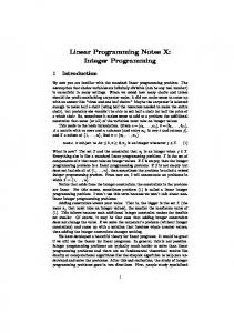
Our property checking framework is illustrated in Figure 2. It consists of three main procedures, namely abstraction, property checking, and refinement. 1

An elementary cycle, also called a basic cycle, is one that cannot be decomposed into smaller cycles.

September 13, 2010

DRAFT


11

Original model

Negated property

Abstraction

ILP problems

Property checking

Yes

Counterexamples

Refinement

Fig. 2.

•

An ILP-based property checking framework for asynchronous reactive systems.

The aim of the abstraction procedure is to encode the checking of the considered property into an ILP problem. The abstraction procedure is conservative, i.e., it keeps all possible behavior of the original system and may introduce some behavior that is not allowed in the original system. The resulting imprecision is unavoidable for the properties whose checking problems are undecidable for infinite state systems.

•

The property checking procedure solves the ILP problems constructed by the abstraction procedure, and interprets the results. In case solutions to the ILP problems are found, it constructs counterexamples from the ILP solutions to illustrate certain property violating scenarios. Counterexamples constructed in our framework are different from those in the context of explicit state model checking. In our setting, a counterexample does not give directly an erroneous execution of the system, but only specifies some constraints or patterns that apply to a potentially infinite set of property violating executions. More precisely, a counterexample indicates which cycles are to be repeated infinitely often in a property violating execution.

•

A refinement procedure is necessary to improve the accuracy of the analysis by recovering information lost during the abstraction. Following the idea in [14], the abstraction refinement that we propose is guided by the counterexamples that we obtain.

The whole checking procedure is iterative, which corresponds to the loop in Figure 2 through the property checking, counterexamples, and refinement blocks: Given a system, for reasons September 13, 2010

DRAFT


12

of efficiency a relatively coarse abstraction is constructed during the first iteration of our checking approach. The model may be too coarse, and a counterexample may be constructed which does not correspond to any real execution of the original system. In this case certain information of the original system is recovered in order to exclude the spurious behavior that the counterexample corresponds to. The property is then checked on the refined abstraction in the next iteration. The model is gradually refined in this way until either it is precise enough to verify the property or the abstraction cannot be refined anymore. IV. C HECKING BUFFER B OUNDEDNESS We present a buffer boundedness test in the proposed ILP-based property checking framework. The unboundedness of the message buffers in a system model can have several negative effects. First, if the model represents a software design, the unboundedness of one or more of the message buffers hints at a possible design fault: The unbounded buffers may result in buffer overflows or losses of messages in the implementation of the design. Second, buffers with unbounded capacity impede automated finite state analyzeability since they induce an infinite state space that renders state space exploration incomplete in finite time. One commonly observes that in a system model where buffers have unbounded capacities, the buffer occupancy may still be bounded by some small constant k because of the particular dynamics of the system. If this is the case, then one can safely replace the unbounded buffers by k-bounded buffers without changing the behavior of the system. Furthermore, the model with k-bounded buffers is now analyzable by finite state verification techniques once other sources of infiniteness (infinite data domains, unbounded number of processes) are ruled out. Since buffer boundedness is undecidable for asynchronous reactive systems the proposed analysis will remain incomplete. Nevertheless, the test is efficient and scales to realistic models of large size, as we will show in the sections on complexity (see the end of Section IV-C) and on experimental results (Section VIII-A). A. Overview of the Boundedness Test We first define formally the buffer boundedness property. Definition 1: Given an asynchronous reactive system, a message buffer b in the system is bounded if and only if there exists a natural number k such that, in any reachable configuration of the system, the buffer b contains no more than k messages. If no such k exists, then b is

September 13, 2010

DRAFT


13

unbounded. The system is bounded if and only if all the buffers are bounded. The system is unbounded if and only if at least one buffer is unbounded. We propose a boundedness test based on ILP solving. The test makes use of a series of abstraction steps that leaves us with an over-approximating abstraction given as an independent cycle system. Boundedness for independent cycle systems can be determined efficiently using ILP solving techniques. The test can also estimate an upper bound for each individual message buffer in case the system is bounded. By the very nature of over-approximations, not every bounded system can be detected as such by this method and the obtained bounds are not necessarily optimal. The underlying idea of our boundedness test is to determine whether it is possible to combine the cyclic executions of a system such that the filling of at least one message buffer can be “blown up” in an unbounded way. B. Abstraction Each abstraction level corresponds to a computational model for which complexity results for the boundedness problem are either known or provided by our work. We show how the complexity of the boundedness problem can be reduced by each abstraction step. The goal of our conceptual abstraction is to arrive at a data structure that allows us to reason about the aggregate message passing effects of control flow cycles using linear combination analysis. Level 0: Promela. We start with a model described in Promela or other modeling languages for asynchronous reactive systems. For the model, boundedness is undecidable since Promela without buffer capacity bounds is expressive enough to simulate Turing machines and boundedness can be reduced to the halting problem of Turing machines [13]. Level 1: CFSM Systems. First, we abstract from the program code in the model, and obtain an over-approximating CFSM system. The code abstraction retains only the finite control structure of the model and the message passing behavior, which we will discuss in details in Section VI. For CFSM systems, it has been shown that boundedness is undecidable [13]. As an example, the model in Figure 1 is transformed into the CFSM system as shown in Figure 3 by discarding all assignments, condition statements, and other statements except message sending and receiving statements. The state machine corresponding to the init process carries no statements at all since it never sends nor receives any messages. Level 2: Parallel-Composition-VASS. In the next step we abstract from the order of messages in the buffers and consider only the number of messages of any given type. For example, the buffer with contents abbacb would be represented by the integer vector September 13, 2010

DRAFT


s11

14

s21

ts[0]!req

t2

t4

s12

ts[1]!rel

s22

tc[0]?ack

s13

r5

tc[0]!ack

tc[1]?ack

r4

r3

r6

ts[1]?req

t1

tc[1]!ack

ts[0]?rel

ts[1]?rel

t3

t5

s23

client(0)

Fig. 3.

r2

ts[1]!req ts[0]?req

ts[0]!rel

r1

client(1)

server()

init

The abstract CFSM system of the Promela model in Figure 1.

(2, 3, 1), representing 2 messages of type a, 3 messages of type b and 1 message of type c. Consequently, no distinction can be made at this level between abbacb and bbbaac that are both represented by the same integer vector. In this way we also abstract from the order of message sending and receiving events in a transition and use an integer vector to denote how many massages of each type are sent or received along the transition. We call such an integer vector an effect vector. A positive component in an effect vector denotes the number of sent messages of the corresponding type, while a negative component denotes the number of received messages of the corresponding type. Consider the CFSM system in Figure 3. Table I shows how message types correspond to different components in effect vectors. Consequently, the transition from the state s11 to the state s12 has the effect vector h1, 0, 0, 0, 0, 0i because it sends a req messages to the buffer ts[0]. The transition from s12 to s13 has the effect vector h0, 0, 0, 0, −1, 0i since it receives an ack messages from the buffer tc[0]. We will discuss how to identify message types in Section VI-A. Effect vector component

Message Type

Effect vector component

Message Type

Effect vector component

Message Type

1st

req in ts[0]

3rd

req in ts[1]

5th

ack in tc[0]

2nd

rel in ts[0]

4th

rel in ts[1]

6th

ack in tc[1]

TABLE I M ESSAGE TYPES AND THEIR CORRESPONDING EFFECT VECTOR COMPONENT.

For the purpose of complexity analysis it is helpful to relate the obtained abstraction to the theory of Petri nets [56]. The numbers of messages in any buffer can be represented by the number of tokens in Petri net places. We then obtain a vector addition system with states (VASS) [11]. The control states correspond to the states of the processes of the CFSM systems September 13, 2010

DRAFT


15

and the Petri net places represent the integer vectors approximating buffer contents. More exactly, we obtain a parallel-composition-VASS. This is a VASS whose finite-control is the parallel composition of several finite state machines. The boundedness problem for parallelcomposition-VASS is to determine, given an initial configuration c0 , whether the system is bounded with respect to c0 . This problem is polynomially equivalent to the boundedness problem for Petri nets, which is EXPSPACE-complete [73]. Level 3: Parallel-Composition-VASS with Arbitrary Initial Tokens. We now abstract from activation conditions of cycles in the control-graph of the parallel-composition-VASS. Any combination of control flow cycles in the system has a minimal activation condition, i.e., a minimal number of tokens needed to get it started. In principle, it is decidable if there is a reachable configuration that satisfies these minimal requirements, but this involves solving the coverability problem for Petri nets: given a Petri net, whether there exists a reachable marking which is bigger than a given marking. This problem is decidable, but at least EXPSPACE-hard [28], [50], and thus not practical. So, we assume instead that there are always enough tokens present to start the cycle. By this abstraction, we replace the boundedness problem “Is the system bounded with respect to a given initial configuration?” by the problem of the so-called structural boundedness: “Is the system bounded with respect to any initial configuration?” It has been shown in [47] that the structural boundedness problem for parallel-compositionVASS is co-NP-complete, unlike for standard Petri nets where it is polynomial [28], [54]. The reason for this difference is that an encoding of control states by Petri net places does not preserve structural boundedness, because it is not assured that only one of these places in each part is marked at any time. Furthermore, the co-NP-lower bound even holds if the number of elementary cycles in the control-graph is only linear in the size of the system [47]. Level 4: Independent Cycle System. Finally, we abstract from the fact that certain control flow cycles within one part or among several parts in a VASS system may depend on each other. For example, cycles might be mutually exclusive so that executing one cycle makes another cycle unreachable. Cycles may also rely on each other, i.e., one cannot repeat some cycle infinitely often without repeating some other cycles infinitely often. By abstracting from cycle dependencies, we assume that all cycles are independent and any combination of them is executable infinitely often, provided that the combined effect of this combination on all places is non-negative. In this way we may abstract the VASS system of Level 3 to a set of independent elementary control flow cycles with their aggregate effect vectors. September 13, 2010

DRAFT


16

We call this system an independent cycle system. For the model in Figure 1, the resulting cycle system consists of the following cycles: (1) hs11 , s12 , s13 , s11 i; (2) hs21 , s22 , s23 , s21 i; (3) ht1 , t2 , t3 , t1 i; (4) ht1 , t4 , t5 , t1 i; and (5) hr2 , r3 , r4 , r2 i. Their effect vectors are, respectively, (1) h1, 1, 0, 0, −1, 0i; (2) h0, 0, 1, 1, 0, −1i; (3) h−1, −1, 0, 0, 1, 0i; (4) h0, 0, −1, −1, 0, 1i; and (5) h0, 0, 0, 0, 0, 0i. Note that each cycle has exactly one effect vector in this example. However, in general the abstraction procedure may result in multiple effect vectors for one transition, and a cycle may therefore have more than one aggregate effect vector. For simplicity reasons we assume that each cycle has only one effect vector for the time being. This will however not reduce the generality of the arguments in the remainder of the section. For convenience reasons, given a set of control flow cycles, we refer to a linear combination of the effect vectors of these cycles as a linear combination of cycles. Finally, we point out that we only consider the overall effect of the complete execution of a cycle in the cycle system. A partially executed cycle is regarded as an acyclic path. C. Boundedness Checking A necessary condition for the unboundedness of a system can be given in terms of the resulting independent cycle system. Theorem 1: If an asynchronous reactive system is unbounded, then there exists a linear combination of cycles in the resulting independent cycle system such that the aggregate effect of the linear combination is positive. Formally, let {vi } be the set of cycle effect vectors, P the system is unbounded if there exists a linear combination xi vi such that (1) every P component in xi vi is non-negative; and (2) at least one component is positive. Intuitively, a positive linear combination of cycles corresponds to a combined effect of control flow cycles that sends at least one message without consuming any messages. Some message buffers will then be flooded by repeating the execution of this combination of cycles. We give the proof in the following that the above theorem gives indeed a necessary condition for unboundedness, which implies the soundness of our boundedness test. In order to prove Theorem 1, we first need the following auxiliary lemma. Lemma 1: For any infinite sequence of integer vectors of same dimension s = h¯ v1 , v¯2 , . . . i, if there exists an integer vector ¯b such that v¯i ≥ ¯b holds for each i, then there is an infinite subsequence h¯ vu1 , v¯u2 , . . . i of s such that v¯ui ≤ v¯uj holds for all ui < uj . Moreover, if s is unbounded, i.e., there exists no integer vector b¯m such that b¯m > v¯i for each i, then there is an infinite subsequence h¯ vw1 , v¯w2 , . . . i of s such that v¯wi < v¯wj holds for all wi < wj . September 13, 2010

DRAFT


17

Proof: We prove the lemma using the induction on the dimension k of the vectors in the sequence. Induction base: Let k = 1. Then, s is actually a sequence of integers hv1 , v2 , . . . i bounded below by b. By contradiction, we assume that there is no infinite non-decreasing subsequence of s. Then, there must exist an upper bound b′ such that vi ≤ b′ for every i. Because there are only finitely many integers v such that b ≤ v ≤ b′ , there must exist infinitely many elements in s that are equivalent. These elements form a non-decreasing subsequence of s, which contradicts the assumption that there is no such subsequence. Induction step: Assume that the lemma holds for all sequences of integer vectors of dimension k, and that s consists of vectors of dimension k + 1. Let trunc(¯ vi ) be an integer vector of dimension k constructed from v¯i in s such that trunc(¯ vi )j = v¯ij for each 1 ≤ j ≤ k. According to the induction assumption, we can select an infinite subsequence s′ of s: h¯ vw1 , v¯w2 , . . . i such that trunc(¯ vwi ) ≤ trunc(¯ vwj ) holds for all wi < wj . The (k + 1)th components of all elements in s′ form an infinite sequence of integers, from which we can select an infinite non-decreasing subsequence of integers h¯ vuk+1 , v¯uk+1 , . . . i, based on the 1 2 argument for the induction base. Apparently, h¯ vu1 , v¯u2 , . . . i satisfies the property that v¯ui ≤ v¯uj holds for all ui < uj . Finally, it is obvious that an infinite subsequence of strictly increasing vectors exists if s is unbounded, which can be proved similarly as above using an induction on the vector dimension k. Now we prove Theorem 1. Proof: It is equivalent to prove the following: Given a finite set of integer vectors v¯1 , . . . , v¯n of the same dimension, say m, the two conditions below are equivalent. •

Condition C1: There exists no xi ∈ N (1 ≤ i ≤ n) such that2 n X

xi v¯i > ¯0.

(1)

i=1 •

Condition C2: For any vector v¯, there exists a vector ¯b such that, for all xi ∈ N (1 ≤ i ≤ n), v¯ +

n X i=1

2

xi v¯i ≥ ¯0 → v¯ +

n X

xi v¯i ≤ ¯b.

(2)

i=1

We use ¯ 0 to denote an all-zero vector where the dimension of the vector is clear from the context.

September 13, 2010

DRAFT


18

Let f (x1 , . . . , xn ) := v¯ + x1 v¯1 + · · · + xn v¯n . We first prove C1 → C2 by contradiction and assume that there exists some k such that no upper bound exists for f (¯ x)k under the condition f (¯ x) ≥ ¯0. This implies that there exists an infinite sequence of non-negative vectors ci )k = +∞. sc = h¯ c1 , c¯2 , . . . i of dimension n such that (1) f (¯ ci ) ≥ ¯0 and (2) limi→∞ f (¯ Following Lemma 1, we may select from sc an infinite subsequence sd = hd¯1 , d¯2 , . . . i such that f (d¯i )k is strictly increasing. Again, from sd we can select an infinite subsequence se = h¯ e1 , e¯2 , . . . i such that f (¯ ei ) is strictly increasing. Moreover, from se we can select an infinite strictly increasing subsequence sg = h¯ g1 , g¯2 , . . . i. From sg we select arbitrarily two elements g¯i and g¯j such that g¯i < g¯j . Based on the ¯ = g¯j − g¯i > 0 and construction of sg , we know that f (¯ gi ) < f (¯ gj ). It is easy to see that h Pn ¯ p Pn ¯ p ¯p = f (¯ gj ) − f (¯ gi ) > 0. Therefore, p=1 h · v¯p is a non-negative solution for p=1 h · v Inequality 1, which results in a contradiction. Second, we prove that C2 → C1 by contradiction and assume that there exists a non-negative vector c¯0 such that f (¯ c0 ) > ¯0. Then we can construct an infinite sequence h¯ c1 , c¯2 , . . . i where c¯i = i · c¯0 . We can easily see that f (¯ ci ) is strictly increasing and no upper bound therefore exists for f (¯ ci ), which leads to a contradiction. The checking of the unboundedness condition can easily be encoded into an ILP problem. Given a system, suppose that the cycles c1 , ..., cm form the resulting independent cycle system together with their respective effect vectors e1 , ..., em , all of which are of dimension n. The ILP problem representing the unboundedness condition is the following:

m X

xj ≥ 0 for each

1≤j≤m

(3)

xj · ekj ≥ 0 for each

1≤k≤n

(4)

j=1 m X n X

xj · ekj > 0

(5)

j=1 k=1

where each xj corresponds to the cycle cj and ek denotes the k-th component of the effect vector e. In the above ILP problem, Inequality (3) requires all the coefficients xj to be non-negative since any linear combination of cycles can contain only natural coefficients. Inequality (4) only requires all the linear combination of cycles to be non-negative. The positivity of combinations is then enforced by Inequality (5).

September 13, 2010

DRAFT


19

If the above ILP problem has no solution for xj values, then the original system must be bounded. Otherwise, the original system is not necessarily unbounded because the unboundedness condition given above is only a necessary but not sufficient condition. The unboundedness could simply be due to the coarseness of the over-approximation. Thus, this test yields an answer of the form “BOUNDED” in case no positive linear combination of cycles exists, and “UNKNOWN” if such a linear combination exists. For the example of Figure 1, we obtain the following boundedness determination ILP problem:

x1 − x3 ≥ 0

(6)

x1 − x3 ≥ 0

(7)

x2 − x4 ≥ 0

(8)

x2 − x4 ≥ 0

(9)

−x1 + x3 ≥ 0

(10)

−x2 + x4 ≥ 0

(11)

x1 + x2 − x3 − x4 > 0

(12)

xi ≥ 0

(13)

One can easily see that the above ILP problem is infeasible. We can therefore conclude a “BOUNDED” verdict for the model. The ILP encoding of the unboundedness condition may result in redundant repetitions of some linear constraints, as can be seen in the above example. These repetitions can easily be discovered syntactically and then be removed. For illustration purposes, we do not remove these repetitions. Complexity. We show that our boundedness test has a polynomial complexity with respect to the number of cycles in the system. Given a system, suppose that there are n message types and m cycle effect vectors in the resulting independent cycle system. Then, the size of the boundedness determination ILP problem is bounded by (m + n + 1) × m. Because the number of cycle effect vectors m is linear in the number of control flow cycles, the size of the ILP problem is polynomial in the number of cycles. Even though there may be exponentially many elementary cycles in a system, we observe that the control flow graphs derived from realistic models of asynchronous reactive systems are normally very sparse, and

September 13, 2010

DRAFT


20

the number of elementary cycles in them is normally polynomial, rather than exponential. Finally, in spite of the NP-completeness of solving general ILP problems, any ILP problem generated in our test to determine boundedness has a special property to make it polynomial time solvable: For each inequality in the ILP problem, the left-hand side does not contain any constant items, and the right-hand side is 0. Such an ILP problem is called a homogeneous ILP problem, and can be solved in polynomial time as follows: We turn the ILP problem into an LP problem by dropping the integrity restriction on the variables. Then, we can solve the LP problem to obtain a rational solution, which is known to be computable in polynomial time [65]. Next, we compute the least common denominator of all the variable values in the rational solution, which is also possible in polynomial time [20]. We can obtain an integer value for each variable by multiplying the rational solution of the variable with the least common denominator. D. Estimating Buffer Bounds A more refined problem is to compute upper bounds on the lengths of individual buffers in the system. Since normally not all buffers can reach maximal length simultaneously, the analysis is done individually for each buffer b. Note that any finite execution of a system can be decomposed into a cyclic part and an acyclic part starting from the initial configuration of the system. The effect of the cyclic part can be denoted as a linear combination of cycles. For each process in the system, we can compute the least upper bound on the effects of all possible acyclic paths in the process since there are only finitely many acyclic paths. Then, the acyclic part effect of the whole system is bounded by the sum of the upper bound of each process. Now, the computation of buffer bounds is to maximize the contribution from the cyclic part. Given a system, suppose that the cycle effect vectors in the resulting independent cycle system are e1 , ..., em . Let a denote the upper bound of the acyclic part effects of the whole system. We encode the buffer bound computation for a buffer b into an ILP problem as follows. Let I contains all the indices of the effect vector components that correspond to types of messages exchanged in the buffer b. max : constraint :

P

P P ak + k∈I i xi · eki P ¯ a+ m i=1 xi · ei ≥ 0

k∈I

xi ≥ 0 for all i ∈ {1, ..., m}

September 13, 2010

(14) (15) (16)

DRAFT


21

The above ILP problem is to maximize the objective function, representing the number of messages in the buffer b, against the constraint stating that there cannot be a negative number of messages at any time. In the example of Figure 1, the upper bounds on the acyclic path effects of the processes client(0), client(1), server(), and init are respectively h1, 0, 0, 0, 0, 0i, h0, 0, 1, 0, 0, 0i, h0, 0, 0, 0, 1, 1i, and h0, 0, 0, 0, 0, 0i. So, the upper bound on the acyclic part effects of the whole system is the sum h1, 0, 1, 0, 1, 1i. The ILP problem to compute the upper bound for the buffer ts[0] is as follows:

max : 1 + 2x1 − 2x3

(17)

1 + x1 − x3 ≥ 0

(18)

0 + x1 − x3 ≥ 0

(19)

1 + x2 − x4 ≥ 0

(20)

0 + x2 − x4 ≥ 0

(21)

1 − x1 + x3 ≥ 0

(22)

1 − x2 + x4 ≥ 0

(23)

xi ≥ 0

(24)

The computed upper bound for ts[0] is 3 while the actual bound is 2. This shows that our buffer bound estimation method is over-approximating and may deliver a larger bound than the actual one. Note also that the buffer bound estimation ILP problem is no longer homogeneous and its solving may hence require exponential time. V. C HECKING L IVELOCK F REEDOM The main characteristic of a reactive system is that of maintaining an ongoing activity of consuming, processing and producing information. One salient property that any correct reactive system must satisfy is deadlock freedom, i.e., the execution of the system is nonblocking. However, a system may be free of deadlock and yet it does not progress in executing its tasks. For example, two components of a system may keep exchanging internal messages with each other and never respond to the outside world. Such a situation is referred to as livelock. The freedom from livelock is highly desirable since it is important to ensure that

September 13, 2010

DRAFT


22

every so often the environment will receive output from the system. We formally define livelock and livelock freedom for Promela models as follows. Definition 2: Given a Promela model, we identify in its control flow graphs a set of local transitions as progress transitions. A livelocked execution is an infinite execution in which all the progress transitions are taken only a finite number of times. The system is free of livelock if no livelocked executions exist. Livelock freedom is a liveness property. We have shown in [45] that it is undecidable for infinite state systems. Consequently, our test is inevitably incomplete. We outline the method as follows. Given a system and a set of predetermined progress transitions, we first carry out the same sequence of abstraction steps as for the boundedness test, which transforms the system into a set of independent control flow cycles with their effect vectors. We collect all progress cycles as those that contain at least one of the progress transitions. We give a necessary condition for the existence of a livelocked execution in terms of the cycle system and the progress cycles. We encode this condition into a homogeneous ILP problem whose size is polynomial in the number of cycles. If the resulting ILP problem has no solution then the necessary condition cannot hold, which implies livelock freedom. On the other hand, if the resulting ILP has solutions then the system may or may not be livelock free, which corresponds to the incomplete side of our test. In the remainder of this section we mainly explain how the necessary condition for a livelock is encoded in an ILP problem. The underlying idea of our test is that a system is livelock free if at least one progress cycle is repeated infinitely often in any infinite execution. Let c1 , . . . , cn be the set of control flow cycles in the corresponding independent cycle system, and cj1 , . . . , cjm (j1 , . . . , jm ∈ {1, . . . , n}) be the set of progress cycles. Let ei denote the effect vector of the cycle ci . We use the following ILP problem to characterize a necessary condition for the existence of a livelocked execution, i.e., an infinite execution in which any progress cycle can be repeated only a finite number of times. n X

xi · ei ≥ ¯0

(25)

n X

xi > 0

(26)

xji = 0

(27)

i=1

i=1 m X i=1

September 13, 2010

DRAFT


23

xi ≥ 0

for each i

(28)

In the above inequalities, each integer variable xi denotes the number of times that the cycle ci is repeated in a linear combination of cycles. These variables may have only non-negative values as imposed by the inequalities (28). The inequality (25) requires a linear combination of cycles to consume no messages. Thus, an infinite repetition of such a combination is possible since it does not run out of any type of messages. The inequality (26) excludes a trivial combination in which no cycle is executed at all. The inequalities (25) and (26) together give a necessary condition for the existence of infinite executions. The inequality (27) then excludes any progress cycle cji from a linear combination. Consequently, this condition excludes any progress cycle from being repeated infinitely often in any infinite execution. Note that the above ILP problem is also homogeneous and thus polynomial time solvable. We prove the soundness of our livelock freedom test as follows. Theorem 2: Given a Promela system and a predetermined set of progress transitions, if the livelock freedom test determines the system to be free of livelock, then the system is actually free of livelock. Proof: If the system is proved to be free of livelock by our method, then there exists no positive linear combination of effect vectors of non-progress cycles since there is no solution to the ILP problem described by the inequalities (25–28). By Theorem 1, we can see that any execution of the system in which only non-progress cycles are repeated infinitely often is bounded. By contradiction, we assume that the Promela system has a livelocked execution r. All the progress cycles are hence repeated only a finite number of times in r. Then there exists a particular point of time t in r after which only non-progress cycles are executed. Furthermore, we have shown above that r is bounded. Note that any process in the system has only finitely many local states. Consequently, there will be only finitely many reachable configurations of the system after t in r. Furthermore, since r is an infinite execution, there must be two distinct points of time t1 and t2 after t at which the system reaches one same configuration. The finite segment of execution between t1 and t2 can be represented as a linear combination of executions of non-progress cycles. The aggregate effect vector of this segment is however an all-zero vector. This contradicts the fact that no solution exists for the ILP problem described by the inequalities (25–28), i.e., there is no non-negative linear combination of non-progress

September 13, 2010

DRAFT


24

cycles. Consider the model in Figure 1. Let the only progress transition be the receipt of an ack message in the process client(0). Then, we have only one progress cycle as the one in client(0). We can build the following ILP problem for determining livelock freedom:

x1 − x3 ≥ 0

(29)

x1 − x3 ≥ 0

(30)

x2 − x4 ≥ 0

(31)

x2 − x4 ≥ 0

(32)

−x1 + x3 ≥ 0

(33)

−x2 + x4 ≥ 0

(34)

x1 + x2 + x3 + x4 + x5 > 0

(35)

x1 = 0

(36)

xi ≥ 0

(37)

We can easily obtain a solution to the above ILP problem as x5 = 1 while xi = 0 where i 6= 5. As a consequence we cannot prove livelock freedom for the example system. In Section VII, where we will re-visit this example, we will show how to construct counterexamples from such an ILP solution, and explain how to perform abstraction refinement based on the constructed counterexamples. VI. C ODE A BSTRACTION As the first abstraction step in both boundedness and livelock freedom tests, the goal of code abstraction is to construct a CFSM system that over-approximates the behavior of the original model. Since CFSM systems only specify message passing behavior, the focus of our code abstraction is on determining the message passing effects of a model. For abstracting Promela models, we have considered issues including (1) the identification of message types; (2) variable dependencies; (3) process replications; (4) buffer assignments; (5) buffer arrays, and (6) unbounded proctype instantiations, among others. The abstraction of Promela code has been fully automated. Due to space limitations we are unable to discuss the solutions to all the above mentioned problems in this paper. For the purpose of illustration September 13, 2010

DRAFT


25

we choose to explain in detail how we identify message types in Promela models in Section VI-A, and sketch how we approximate cycle effect vectors in Section VI-B. Discussions of other abstraction solutions can be found in [49], [72]. A. Identifying Message Types We formally define a message type as a subset of messages exchanged in a model. Identifying too few message types may lead to an imprecise property checking. Identifying too many message types on the other hand may drastically increase the size of the property determination ILP problems, which makes the property checking inefficient [72]. We propose here a message type identification method which is optimal in the sense that no other identification method can lead to a more precise property checking. Meanwhile our method attempts to minimize the number of identified message types by ruling out messages that can never appear in the model. The first intuition of the optimal method is that we only need to distinguish two messages if they can be distinguished by a message receiving statement in the model. As an example, if ch?req, 5 is in a model, then messages (ch, req, 5) are distinguished from those req messages containing a different value than 5, and we therefore need to identify the message type {(ch, req, 5)}. On the contrary, if ch?req, x is the only statement to receive req messages from ch in the model where x is an integer variable, then there is no need to distinguish different values for the second component of req messages. In this case, a message type {(ch, req, x)|x ∈ I} is sufficient where I is the set of all integers. The second intuition is that we need to identify a message type only if it can be possibly exchanged in the model. We explain the optimal message identification method as follows. We use FINAL to denote the set of message types identified by our method. First, we identify a set of message types SENT including, for each message sending statement, the subset of messages that can be possibly sent by the statement. For instance, for the model in Figure 1, the resulting set SENT is {(ts[0 ], req)}, {(ts[0 ], rel )}, {(ts[1 ], req)}, {(ts[1 ], rel )}, {(tc[0 ], ack )}, {(tc[1 ], ack )}. Next, we identify a set of message types RECEIVE including, for each message receiving statement, the subset of messages that can be possibly received by the statement. In our example, the set RECEIVE is {(ts[0 ], req)}, {(ts[0 ], rel )}, {(ts[1 ], req)}, {(ts[1 ], rel )}, {(tc[0 ], ack )}, {(tc[1 ], ack )}. In the last step, we first add every message type m in RECEIVE to FINAL. Then, let ALLR be the union of all message types in RECEIVE . For each message type m in SENT , September 13, 2010

DRAFT


26

if m′ = m − ALLR is not empty, then we also add m′ to FINAL. In our example, the final set of identified message types is {(ts[0 ], req)}, {(ts[0 ], rel )}, {(ts[1 ], req)}, {(ts[1 ], rel )}, {(tc[0 ], ack )}, {(tc[1 ], ack )}, which is identical to RECEIVE since all sent message types in SENT are covered by the collection of the received message types. The above message type identification is optimal with respect to the necessary condition for unboundedness given in Theorem 1: Let L1 be the boundedness determination ILP problem resulting from the optimal message type identification method, and L2 be the ILP problem resulting from any other identification method. It can be shown that, whenever L2 is infeasible, L1 is feasible as well [72]. B. Determining Cycle Effect Vectors

1 mtype = { ack , r e j } ; 2

...

...

3 a c t i v e p r o c t y p e Medium ( ) { 4

mtype msg ;

5

do

6

...

7

: : s2m ? msg −> m2c ! msg

...

8

od

9 }

Fig. 4.

A simple Promela model.

The message passing effect of a control flow cycle is the aggregate effect of all transitions along the cycle. However, a transition may have more than one effect vector, e.g., because of the use of variables in the transition. As a safe over-approximation, we can take all possible combinations of the effect vectors of the transitions along the cycle. Unfortunately, the number of combinations can be exponentially many and therefore tremendously increases the size of the property checking ILP problems. However, not all combinations of transition effect vectors are possible due to dependencies among statements. Consider Line 7 in the model in Figure 4. The statement s2m?msg may receive an ack or a rej message, and the statement m2c!msg may send an ack or a rej message. The total number of combinations is thus 4. However, we can easily see that the variable msg used to store received messages is unmodified before being forwarded. Therefore, the combination of receiving an ack message and then sending a rej message is impossible. As a solution to exclude impossible cycle September 13, 2010

DRAFT


27

effect vectors, we devise a method to capture dependencies among message sending and receiving statements. The intuitive idea is as follows. For any message sending statement s that has more than one effect vector, we first collect all variables occurring in the statement as the set Var s . Then, we determine the longest acyclic path p reaching s such that any state along p has at most one incoming messages, i.e., the longest path that can be consecutively executed before the statement s is reached. Next, for each variable x in Var s , we determine the closest message receiving statement s′ to s on p such that x is used to store a component of incoming messages and x is unmodified between s and s′ . If s′ exists, then we can obtain a dependency of x’s value on the types of messages that s′ receives. In our example, the dependency for msg is the following: (1) msg = ack if and only if s2m?msg receives messages of the type {(s2m, ack )}; and msg = rej if and only if s2m?msg receives messages of the type {(s2m, rej )}. Then, we can use these dependencies to rule out impossible cycle effect vectors such as the one in which {(s2m, ack)} is received but msg = rej is forwarded instead. VII. C OUNTEREXAMPLE -G UIDED A BSTRACTION R EFINEMENT In our ILP based property checking framework, we may obtain a solution to the property determination ILP problem. In this case, we do not know whether the property is satisfied by the system or not. Fortunately, the returned ILP solution may provide useful information about potential property violating behavior. A solution to a property determination ILP problem represents a particular linear combination of cycles such that infinitely repeating this combination without executing other cycles results in a property violation. Therefore, we define a counterexample in our setting as follows. Given a solution to the property determination ILP problem, a counterexample is a set of control flow cycles whose corresponding variables in the ILP problem receive nonzero values in the given solution. Intuitively, a counterexample corresponds to those system executions in which only the cycles in the counterexample are repeated infinitely often, and all other cycles are either repeated only a finite number of times, or not executed at all. Due to the imprecision induced by the abstraction steps that we perform, a counterexample may correspond to no executions of the original system, in which case we call the counterexample spurious. In the end of Section V, we obtain an ILP solution while checking livelock freedom on the model in Figure 1. Based on the above definition, the corresponding counterexample September 13, 2010

DRAFT


28

consists of the only cycle in the init process. The cycle performs the task to create multiple instances of clients. This counterexample is apparently spurious: The execution of the cycle is guarded by the condition i < 2, and every execution of the cycle increases the value of i. So, it cannot be repeated forever by itself. While in the above case we can easily see that the counterexample is spurious, in general it is impossible to determine spuriousness manually. The introduction of spurious counterexamples is a consequence of the conservative abstraction steps that we perform in the course of our buffer boundedness or livelock freedom test. We reconsider each of these abstraction steps to examine which information is removed from models during the step and how significantly it affects the precision of the analysis. a) Code Abstraction: In this step the program code in a model is abstracted away. We lose all the information about how the behavior of the model is constrained by the conditions on variables that are imposed by the program code. Losing such information is very significant because it often depends on the runtime value of a variable whether to send or receive a message, which message to send or receive, and where messages are to be sent or received. We will therefore consider to recover this information during refinement. b) Abstraction from Message Orders: In this step we ignore all information regarding the order of messages in buffers. In particular, we assume that a message is always available to trigger a transition wherever it is in the buffer. This can be too coarse an overapproximation for a model that employs strict FIFO message buffers. However, many models in practice, in particular if they mimic the message passing semantics of the UML sublanguages SDL or UML RT, use a message deferral/recall mechanism. This mechanism stores an arriving message which cannot immediately be processed by the system into a special buffer so that it can be recalled when it is later needed. For this type of models, this abstraction step does not introduce imprecision. c) Abstraction from Activation Conditions: In this step the activation conditions of control flow cycles are abstracted away. We assume that there are always enough messages of the right type available for a cycle to be reachable from the initial configuration of the model. In this way we abstract from the dependency between the acyclic part and the cyclic part of an execution. The loss of the activation conditions of cycles is also significant, especially in the estimation of buffer bounds, as we allow any combination of acyclic path effects and cyclic effects. d) Abstraction from Cycle Dependencies: In this step we abstract from dependencies between control flow cycles. Cycle dependencies may be caused by many reasons, such as September 13, 2010

DRAFT


29

by the program code along control flow cycles, or by the structural characteristics of control flow graphs. Disregarding cycle dependencies means that arbitrary cyclic executions can be combined to form a potentially spurious counterexample. Therefore, this is also a significant source of imprecision. In this paper we will pay special attention to the discovery of cycle dependencies by reconsidering the program code in the original Promela model. We will address other sources of imprecision in future work, especially the dependencies between cycles and acyclic paths. Note that counterexample analysis and abstraction refinement based on cycle dependency discovery is expensive and difficult, as it involves the analysis of program code, e.g., termination proofs and cycle iteration count estimation. Also, as we will see later, the refinement may result in an exponential number of ILP problems to solve. Therefore, we should call the refinement procedure only when necessary, i.e., when a counterexample is found. Furthermore, only those cycles in the counterexample are subject to the dependency analysis in the effort to remove the potential spurious behavior represented by the counterexample. Finally, our refinement methods are incomplete, and it is possible that the spuriousness of a counterexample cannot be determined by our methods. A. Detecting Cycle Dependencies We first define the concept of cycle dependencies. Let IRC (r) denote the set of cycles repeated infinitely often in an execution r. Intuitively, a cycle c depends on a set of cycles S if the infinite execution of c must be accompanied by the infinite executions of some cycles in S. Definition 3: Given a Promela model, a cycle c and a set of cycles S in the model, we call the pair (c, S) a cycle dependency if they satisfy the following conditions: a) c ∈ / S; and b) for any infinite execution r of the model where c ∈ IRC (r), there exists a cycle c′ ∈ S such that c′ ∈ IRC (r). In this case, we say that c depends on S, and that S is a correlated cycle set (CCS) of c. In the above definition, if all the cycles in S are in the same process as c is, then (c, S) is a local dependency. Otherwise, (c, S) is a global dependency. Moreover, if c does not depend on any subset of S, then we say that (c, S) is a minimal dependency. We have shown in [48] that it is undecidable for infinite state systems to determine whether c depends on S for an arbitrary pair of c and S.

September 13, 2010

DRAFT


30

Given a positive integer n, (n, c, S) is called a numerical cycle dependency if (1) (c, S) is a cycle dependency and (2) every n times that c is repeated, one of the cycles in S must be executed at least once. The root cause for cycle dependencies lies in the executability of Promela statements. Given a cycle, if the executability of every statement along the cycle is unconditional, then the cycle can be repeated without interruption forever once the cycle is entered. Such a cycle does not depend on any other cycles. On the contrary, consider a cycle c that contains a statement s whose executability is conditional. If s cannot be continuously enabled forever by only repeating c, then some other cycles need to be executed in order to re-enable s by, e.g., modifying the values of some variables, sending a message etc. In Promela, condition statements and message receiving statements are two kinds of statements with conditional executability. In the following, we illustrate how we can obtain cycle dependencies from condition statements. Other automated cycle dependency detection methods, including those concerning dependencies caused by message receiving statements, are described in detail in [48], [72].

C1 i = 0 (i>2) (i 0

(45)

x1 = 0

(46)

xi ≥ 0

(47)

x5 ≤ 0

(48)

The solving of the above ILP problem leads to a new counterexample as {c2 , c4 } where c2 is the only control flow cycle in the process client(1) and c4 is the cycle in the server that responds to client(1)’s request. Our cycle dependency analysis methods fail to determine any dependencies for the cycles in the counterexample, which reflects the incompleteness of these methods. This results in an “UNKNOWN” conclusion from the livelock freedom test. By manual inspection, we can easily see that the counterexample is indeed real and reveals September 13, 2010

DRAFT


35

the livelocked scenario where the server decides to respond to client(1) only and ignores any message sent from client(0). We show in the following that the above described refinement method preserves the soundness of the property checking methods. We only prove here the case for the buffer boundedness test. The argument for the livelock freedom test can be similarly obtained. Theorem 3: Given a Promela system, if the boundedness test determines the system to be bounded after a refinement using a numerical cycle dependency (m, c, D), then the system is actually bounded. Proof: Without loss of generality, we assume that the boundedness determination ILP problem for a model without refinements is as follows x1 · e¯1 + · · · + xn · e¯n > ¯0

(49)

Suppose that c corresponds a set of effect vectors Ec , and Ec correspond to the set of variables Xc in the above ILP problem. Similarly, we assume that the cycles in D correspond to the set of variables Xd in the above ILP problem. The refinement based on (m, c, D) then results in the following ILP problem: x1 · e¯1 + · · · + xn · e¯n > ¯0 X X xi xi ≤ m xi ∈Xc

(50) (51)

xi ∈Xd

Because buffer boundedness is proved for the model, the above ILP problem has no solutions. Given any vector e¯, we now prove that (*) if the above ILP problem has no P solutions, then there exists a vector ¯b such that f (x1 , . . . , xn ) = e¯ + ni=1 xi · e¯i ≥ 0 → P P f (x1 , . . . , xn ) ≤ ¯b for all x1 , . . . , xn where xi ∈Xc xi ≤ m xi ∈Xd xi . By contradiction, we assume that there exists no bound. Then, according to the proof of Theorem 1, we can construct a sequence of strictly increasing non-negative integer vectors h¯ c1 , c¯2 , . . . i such that f (¯ ci ) is also strictly increasing and the following is satisfied: Let Ic denote the set of indices j such that xj ∈ Xc , Id denote the set of indices j such that xj ∈ Xd . For any c¯i , we have P P that j∈Xc c¯ji ≤ m j∈Xd c¯ji . Now we select arbitrarily two c¯i and c¯j such that c¯i < c¯j . It is P P easy to see that d¯ = c¯j − c¯i has the property that d¯j ≤ m d¯j . Therefore, d¯ is a j∈Xc

j∈Xd

solution to the ILP problem (50–51). This leads to a contradiction. Now we start to prove the soundness of our refinement method. It suffices to prove that, if the ILP problem above has no solutions, then the model is bounded with the following

September 13, 2010

DRAFT


36

restriction: Every m times that the cycle c is repeated, some cycle in D is executed at least once. By contradiction, we assume that the model is unbounded. Any finite prefix of an execution of the model can be decomposed into an acyclic part and a cyclic part. Because there are only finitely many possible acyclic parts for execution prefixes, there is an upper bound ¯ba on the effect vectors generated by acyclic parts. Furthermore, the cyclic part of an execution prefix can be decomposed into a linear combination of cycles. Consider any finite execution prefix r in which c is executed i times and the cycles in D are executed j times such that i > m · j. We decompose the cyclic part of r into the following two linear combinations of cycles: (1) a linear combination containing m · j times of executions of c, and j times of executions of some cycles from D, and executions of other cycles; and (2) a linear combination containing (i − m · j) times of executions of c. Note that (i − m · j) ≤ m because every m times that c is repeated, one cycle in D has to be executed at least once. Therefore, the effect vector of the second linear combination is bounded by some vector ¯b2 . In the statement (*) above, let e¯ = ¯ba + ¯b2 , and we can see that the first P P linear combination constructed from r satisfies the condition xi ∈Xc xi ≤ m xi ∈Xd xi . We denote by ¯b1 the effect vector generated by the first linear combination. Then, ¯ba + ¯b2 + ¯b1 is a buffer bound for any execution prefix r. Consequently, the model is bounded, which contradicts the assumption. Finally, it should be noted that the homogeneity of a property checking ILP problem is preserved after it is augmented with any inequality representing a numerical cycle dependency. 3) Refinement Using Non-Numerical Cycle Dependencies: When we fail to determine cycle iteration counts, we obtain only non-numerical cycle dependencies. Unfortunately, such dependencies can only be used to refine abstractions for the livelock freedom analysis but not for the boundedness analysis [72]. The intuition is that a non-numerical cycle dependency (c, S) has no bound on how many times c can be repeated without any cycle in the set S to be executed. A non-numerical dependency (c, S) results in two alternative restrictions on the execution of a model, namely (1) the cycle c is not repeated infinitely often, or (2) c is repeated infinitely often and one of the cycles in S is also repeated infinitely often. These two possibilities lead to two sets of inequalities. Suppose that c corresponds to the set of variables Xc in the livelock freedom determination ILP problem, and the cycles in S correspond to the set of

September 13, 2010

DRAFT


37

variables XS . Then, we can encode the first possibility in the following set of inequalities: X xi = 0 (52) xi ∈Xc

and the second possibility in X

xi > 0

(53)

xi > 0

(54)

xi ∈Xc

X

xi ∈XS

Because an ILP problem is essentially a conjunction of linear inequalities and cannot express disjunctions, we need to build two new ILP problems, each augmenting the original ILP problem with one of the two sets above. In order to prove livelock freedom for the original Promela model, we must show that both newly constructed ILP problems have no solutions. As a consequence, each refinement using non-numerical dependencies doubles the number of ILP problems that need to be solved. This may cause an exponential increase in the number of livelock freedom determination ILP problems. We show the soundness of the above refinement procedure in the following. Theorem 4: Given a Promela system, if the livelock freedom test determines the system to be free of livelock after a refinement using a non-numerical cycle dependency (c, D), then the system is actually free of livelock. Proof: Without loss of generality, we assume that the livelock freedom determination ILP problem for a model without refinements is as follows x1 · e¯1 + · · · + xn · e¯n ≥ ¯0 n X xi > 0

(55) (56)

i=1

X

xi = 0

(57)

ei ∈P CE

where P CE is the effect vectors of the progress cycles. Now assume that we use the cycle dependency (c, D) to refine the above ILP problem. Suppose that c corresponds a set of effect vectors Ec , and Ec correspond to the set of variables Xc in the above ILP problem. Similarly, we assume that the cycles in D correspond to the set of variables Xd in the above ILP problem. The refinement based on the cycle dependency

September 13, 2010

DRAFT


38

(c, D) then results in the following two ILP problems: x1 · e¯1 + · · · + xn · e¯n ≥ ¯0 n X xi > 0

(58) (59)

i=1

X

xi = 0

(60)

xi = 0

(61)

x1 · e¯1 + · · · + xn · e¯n ≥ ¯0 n X xi > 0

(62)

ci ∈P C

X

xi ∈Xc

and

(63)

i=1

X

xi = 0

(64)

xi > 0

(65)

xi > 0

(66)

ci ∈P C

X

xi ∈Xc

X

xi ∈Xd

Because livelock freedom is determined for the model, the two ILP problems above have no solutions. It suffices to prove that, if the two ILP problems above have no solutions, then the model is free of livelock with the restriction that if c is executed infinitely often then some cycle in D is also executed infinitely often. By contradiction, we assume that the model has a livelocked execution r. So, after some point of runtime t0 , no progress cycle is executed in r. There are two possible cases for r as follows. First, if after t0 the cycle c is executed at most a finite number of times, then there exists another point of runtime t1 > t0 such that c is no longer executed after t1 . Because all processes in the model have a finite control flow structure, the infinite suffix of r after t1 must contain an infinite number of configurations such that they agree on the local state of each process. We order these configurations by their occurrence in r and obtain an infinite sequence hs1 , s2 , . . . i. Let eff (si ) denote the effect vector that describes the number of messages of each type at si . Note that each eff (si ) is bounded below by the all-zero vector. Following Lemma 1, there exist two configurations si and sj such that i < j and eff (si ) ≤ eff (sj ). The path between si and sj can be decomposed into a linear combination of cycles in which September 13, 2010

DRAFT


39

at least one cycle is executed and neither c nor any progress cycle is executed. Apparently, this linear combination is non-negative, which contradicts the fact that there is no solution to the ILP problem (58–61). Second, if after t0 the cycle c and some cycle c′ ∈ D are executed infinitely often, then we select arbitrarily a configuration s1 at which one execution of c is started. After s1 , we may select another configuration s2 such that (1) s1 and s2 agree on the local state of each process; (2) another execution of c is started at s2 ; and (3) between s1 and s2 at least one execution of c′ is completed. This selection procedure can continue forever because c and c′ are executed infinitely often, which results in an infinite sequence hs1 , s2 , . . . i. Similar to the argument for the first case, there exist two configurations si and sj such that i < j and eff (si ) ≤ eff (sj ). The path between si and sj can be decomposed into a linear combination of cycles in which c is executed, at least one cycle in D is executed, and no progress cycle is executed. Apparently, this linear combination is non-negative, which contradicts the fact that there is no solution to the ILP problem (62–66). VIII. E XPERIMENTAL R ESULTS We implemented the checking of both buffer boundedness and livelock freedom for Promela models in a fully automated prototype tool called Ciclo. It uses the open source linear optimization tool lp solve as its ILP solving engine [4]. All experiments were conducted on an AMD Athlon 64 X2 Dual machine with 896MB memory. We used a broad range of models for experimentation, including distributed applications, embedded systems, election algorithms, consensus algorithms and communication protocols, as shown in Table II3 . These models contain many of the software architectural features that are typical for the domain that we consider, such as dynamic concurrent processes and message passing based synchronization. We hence believe that we are using an unbiased selection of models that allows for a systematic experimental evaluation of our analysis approach. Many of these models possess considerable size and complexity. As an example, the Conway model is among the smallest and simplest models in our collection, whose boundedness was successfully proved by Ciclo. However, its reachable global states are more than 5.9e7 , which is already too large for the SPIN model checker to verify livelock freedom. 3

The i-Protocol and Mobile Handover models were not subjected to our boundedness analysis because they use only

synchronous communication. We did not check livelock freedom for the CMDA-RLP and Sleep-Wakeup models since it was difficult for us to identify proper progress transitions in these two models. September 13, 2010

DRAFT

IEEE TRANSACTIONS ON SOFTWARE ENGINEERING Model

40

# Proctypes

# Running Processes

# Local States

# Local Transitions

# Buffers

CDMA-RLP [3]

2

2

174

228

3

Conway [9]

4

4

25

34

3

CORBA-GIOP [42]

5

8

126

156

12

Credit Recovery [9]

5

11

52

56

8

GARP [57]

7

8

84

141

10

HTTPR-Pull [62]

3

4

207

247

5

i-Protocol [25]

4

4

54

75

4

ITU-T [55]

7

12

190

243

38

Leader Election [7]

2

5

32

41

5

Mobile Handover [7]

6

6

49

62

7

MVCC [69]

6

9

69

83

14

Neilsen-Mizuno [9]

3

11

43

48

5

SIP [61]

5

Indef.

62

86

4

Sleep-Wakeup [6]

4

4

49

60

1

Snooping Cache [7]

7

7

131

189

14

Train Controller [5]

4

5

55

62

10

TABLE II P ROMELA M ODELS ( IN ALPHABETICAL ORDER ).

A. Checking Buffer Boundedness Model

Result

RunTime

Runtime

Runtime

Runtime

Runtime

(Sec.)

Abstraction

ILP Solving

Refinement

Buf. Est.

# Cycles

# Effect

# Message

# ILP

Vectors

Types

Solved

Leader Election

BOUNDED

0.58

0.13

0.03

-

0.39

8

62

20

6

Snooping Cache

BOUNDED

1.81

0.41

0.05

-

1.28

104

104

36

15

CDMA-RLP

BOUNDED

31.89

19.98

0.01

-

11.70

886

1772

4

3

Credit Recovery

BOUNDED

0.19

0.05

0.09

0.03

-

5

14

10

4

Conway

BOUNDED

0.42

0.05

0.2

0.17

-

12

24

7

5

SIP

BOUNDED

2.44

1.63

0.28

-

-

14

2187

34

1

Sleep-Wakeup

UNKNOWN

0.14

0.05

0.03

0.05

-

17

17

1

1

MVCC

UNKNOWN

1.05

0.11

0.19

0.61

-

19

41

30

4

Train Controller

UNKNOWN

0.81

0.16

0.33

0.28

-

10

174

18

2

HTTPR-Pull

UNKNOWN

0.97

0.3

0.13

0.42

-

39

46

7

3

ITU-T

UNKNOWN

1.13

0.5

0.16

0.3

-

54

207

56

2

GARP

UNKNOWN

1.36

0.19

0.36

0.66

-

51

94

19

6

CORBA-GIOP

UNKNOWN

1.44

0.16

0.2

0.97

-

34

38

12

5

Neilsen-Mizuno

UNKNOWN

4.05

1.01

2.05

0.67

-

8

781

55

3

TABLE III E XPERIMENTAL DATA FOR CHECKING BUFFER BOUNDEDNESS USING C ICLO

Table III shows the experimental results and computational performance figures for checking buffer boundedness using Ciclo. Notice that the runtime for checking a model is not directly correlated with the size of the model. Instead, it depends on further factors, such as (1) how much time it needs to perform code abstraction; (2) how large the resulting boundedness determination ILP problem is; (3) how many refinement iterations are taken; (4) how many

September 13, 2010

DRAFT


41

cycle dependencies can be derived; and (5) the number of message buffers for which buffer bounds need to be computed, among others. Consider the models “CDMA-RLP” and “ITUT” which have comparable sizes. The checking of the “CDMA-RLP” model took much longer time than the checking of the “ITU-T” model. The reasons are the following: First, the “CDMA-RLP” model contains much more control flow cycles for which summary effect vectors need to be computed, which again involves costly statement and variable dependency detection to rule out impossible combinations of message passing effects of the transitions along a cycle. Second, buffer bound estimation for the “CDMA-RLP” model needs to solve three ILP problems, each of which is much larger than the boundedness determination ILP problem for the “ITU-T” model. Model

Runtime

# Found

# Found Spurious

# Analyzed

# Lines Of

Constructed

Refinement

Counterexamples

Counterexamples

Cycles

Code

Cycle Dependencies

Credit Recovery

0.03

1

1

1

6

1

Sleep-Wakeup

0.05

1

0

1

6

0

Conway

0.17

4

4

16

48

4

Train Controller

0.28

2

1

19

122

3

0.3

1

0

83

411

2

HTTPR-Pull

0.42

2

1

122

1514

2

MVCC

0.61

4

2

72

307

29

GARP

0.66

5

2

135

550

23

Neilsen-Mizuno

0.67

2

0

34

356

3

CORBA-GIOP

0.97

4

2

61

429

18

ITU-T

TABLE IV R EFINEMENT P ERFORMANCE OF C ICLO FOR B OUNDEDNESS T EST

Table IV shows that, during abstraction refinement, Ciclo scaled quite well with respect to the number and the sizes of the cycles that it analyzed. Even though we can observe that more analyzed cycles and lines of code result generally in longer runtime, the refinement performance also depends on other factors such as how many cycle dependencies are constructed, or how large the analyzed cycles are on average. To better illustrate the scalability of the Ciclo tool, we compare the runtime performance of checking different versions of the same models, as shown in Table V. We observe, for instance, that the runtime doubles when the number of running processes increases from 33 to 63 for the MVCC model. In the Leader Election model, when we increase the number of processes by a factor of 5 from 5 to 25, the runtime increases by a factor of 12.6. When we double the number of processes from 25 to 50, the runtime increases by a factor 4.5. We believe that these numbers are consistent with the polynomial complexity results September 13, 2010

DRAFT


Version

# Running

# Buffer

Processes

42

RunTime

# Effect

# Message

# Counter-

# Spurious

# Detected Cycle

(Sec.)

Vectors

Types

examples

Counterexamples

Dependencies

Leader Election

5 processes

5

5

0.58

62

20

0

0

-

Leader Election

10 processes

10

10

1.45

122

40

0

0

-

Leader Election

15 processes

15

15

2.78

182

60

0

0

-

Leader Election

20 processes

20

20

4.66

242

80

0

0

-

Leader Election

25 processes

25

25

7.33

302

100

0

0

-

Leader Election

30 processes

30

30

10.58

362

120

0

0

-

Leader Election

35 processes

35

35

14.84

422

140

0

0

-

Leader Election

40 processes

40

40

20

482

160

0

0

-

Leader Election

45 processes

45

45

28.08

542

180

0

0

-

Leader Election

50 processes

50

50

33.53

602

200

0

0

-

MVCC

2 users

9

14

1.05

41

30

4

2

29

MVCC

4 users

15

24

1.25

69

54

4

2

29

MVCC

6 users

21

34

1.5

97

78

4

2

29

MVCC

8 users

27

44

1.34

125

102

4

3

15

MVCC

10 users

33

54

2.06

153

126

4

2

29

MVCC

12 users

39

64

2.38

181

150

4

2

29

MVCC

14 users

45

74

2.17

209

174

4

3

15

MVCC

16 users

51

84

3.22

237

198

4

3

29

MVCC

18 users

57

94

3.58

265

222

4

2

29

MVCC

20 users

63

104

4.09

293

246

4

2

30

TABLE V C OMPARISON OF THE RUNTIME PERFORMANCE FOR CHECKING BOUNDEDNESS FOR DIFFERENT VERSIONS OF MODELS .

obtained in Section IV-C. The runtime growth for the MVCC model is flatter than that of the Leader Election model. This is because user proctype instances do not contribute to unbounded behavior, and therefore the increase in the number of user instances has no effect on the abstraction refinement procedure at all. This results in the same amount of runtime for abstraction refinement for different versions of the model, which happens to take up a large portion of the total runtime for each version. As shown in Table III, six out of fourteen models were proved to be bounded by Ciclo, and buffer bounds were estimated for three models. Most estimated buffer bounds are small numbers and, as far as we can tell by manual inspection, close to the actual bounds. For instance, Ciclo determined that each buffer in the “Leader Election” model can contain no more than 6 messages, while the actual bound was determined to be 5. For the other three models whose boundedness was proved, Ciclo was not able to deliver approximate buffer bounds because either abstraction refinement was used or the running processes could not be statically determined during the checking of these models. In these cases our buffer bound estimation method was not able to give a proper upper bound on the message passing effects of all possible acyclic execution parts, and therefore failed to estimate buffer bounds. Ciclo computed an “UNKNOWN” verdict for 8 models. We manually checked their counSeptember 13, 2010

DRAFT


43

terexamples after no spuriousness could be determined by the tool. For the “Sleep-Wakeup” and “MVCC” models, our inspection revealed that their counterexamples are real. For the 6 models appearing in the bottom section in Table III, none of the reported counterexamples could be determined as real. In the case of the “GARP” model, the executability of a control flow cycle is guarded by the emptiness of a message buffer. However, since we abstract from activation conditions of cycles, our boundedness analysis is no longer able to test buffer emptiness. This results in the failure of Ciclo to determine spuriousness of the last counterexample that it found. Table III highlights the importance of cycle dependency analysis to detect and rule out spurious counterexamples. We found that most computed cycle dependencies are either minimal, or precise enough for determining counterexample spuriousness. As an example, in the boundedness checking for the “MVCC” model Ciclo found a counterexample consisting of a cycle that is executable only if the Updater process is allowed to process inputs. This is indicated by the true value of a flag variable called canProcessInput. The execution of this cycle however sets the flag to false. While analyzing this counterexample, Ciclo successfully detected a precise CCS for the above mentioned cycle, which contains the only cycle that sets the flag canProcessInput back to true. This cycle dependency was then used to rule out the counterexample in our example. However, we also noticed that our cycle dependency detection method generated imprecise dependencies for some models and consequently failed to refine the abstractions. As an example, the checking of the “HTTPRPull” model reported a counterexample in which there is a cycle that is executable if the process crash counter is not larger than 2. However, Ciclo constructed an imprecise CCS, among which some cycles may even further increase the process crash counter. This coarse cycle dependency could not help to rule out the spurious behavior in which the process crash count is larger than 2 forever while the mentioned cycle in the counterexample can still be repeated infinitely often. Even if Ciclo returned ”UNKNOWN” in numerous cases, the fact that our analysis returns diagnostic information in the form of counterexamples greatly helped in understanding potential threats to the unboundedness of the considered models. Further increasing the precision of our analysis is an objective for future research.

September 13, 2010

DRAFT


Result

RunTime

# ILPs

(Sec.)

44

# Counter-

# Spurious

# Detected Cycle

examples

Counterexamples

Dependencies

SPIN Runtime

# Visited Global States by SPIN

Credit Recovery

LIVELOCK-FREE

0.17

2

1

1

1

9.67 sec.

1.3e6

Conway

LIVELOCK-FREE

0.42

5

4

4

4

>> 13 hours

>> 5.9e7

MVCC

LIVELOCK-FREE

0.81

4

3

3

3

4.88 sec.

780580

GARP

LIVELOCK-FREE

1.71

6

5

5

5

204 sec.

1.1e6

Mobile Handover

UNKNOWN

0.28

2

1

0

1

0.015 sec.

43

Snooping Cache

UNKNOWN

2.17

4

4

3

3

0.016 sec.

32

Leader Election

UNKNOWN

0.55

2

1

0

1

-

-

Train Controller

UNKNOWN

0.58

2

2

1

1

-

-

i-Protocol

UNKNOWN

0.53

5

4

1

4

-

-

ITU-T

UNKNOWN

0.73

1

1

0

0

-

-

CORBA-GIOP

UNKNOWN

2.02

4

3

2

3

-

-

Neilsen-Mizuno

UNKNOWN

2.19

2

2

1

1

-

-

SIP

UNKNOWN

4.33

3

2

0

2

-

-

HTTPR-Pull

UNKNOWN

3.67

5

4

2

4

-

-

TABLE VI E XPERIMENTAL DATA FOR CHECKING LIVELOCK FREEDOM USING C ICLO

B. Checking Livelock Freedom Table VI shows the experimental results of checking livelock freedom using Ciclo. We compare the runtime performance of Ciclo and the SPIN model checker for checking livelock freedom for the first six models in Table VI. For the four models whose livelock freedom was proved by Ciclo, SPIN either took much longer time to prove the property or, in case of the “Conway” model, did not reach any conclusion after running for more than 13 hours. As another example, when we increased the number of user processes from 2 to 4 in the “MVCC” model, SPIN could not finish the checking after 1 hour before we ran out of patience and terminated the model checker. For the models “Mobile Handover” and “Snooping Cache” we were able to establish manually, based on the counterexamples provided by Ciclo, that they were indeed livelocked. This was confirmed by SPIN, and interestingly in these cases SPIN took a lot less runtime to produce the proof by model checking than it took Ciclo to compute counterexamples. For the final group of eight protocols we were unable to establish manually whether these models were actually livelocked, and we therefore did not perform a systematic experimental comparison with SPIN. However, for the “i-Protocol” SPIN can prove livelock freedom in a fraction of a second while Ciclo failed after not being able to determine spuriousness for some counterexamples that it constructed. Note that the difference of the columns “Counterexamples” and “Spurious Counterexamples” gives the number of counterexamples that could not be proven spurious, and hence at the potential for improving the counterexample refinement procedure that we use. September 13, 2010

DRAFT


45

The imprecision of our livelock freedom analysis reflects the coarseness of our code abstraction and cycle dependency determination techniques, which need to be improved in future work. The experimental results show that Ciclo can be used as a complementary tool to the SPIN model checker for the checking of livelock freedom, especially when the model being checked is too large for SPIN to reach conclusion within a reasonable amount of time. IX. C ONCLUSION We have presented a property checking framework for buffer boundedness and livelock freedom analysis applicable to infinite state asynchronous reactive systems given as Promela models. Since these two properties are undecidable for infinite state systems, the property checking methods that we proposed are inevitably incomplete. We proposed an automated, incomplete abstraction refinement method in order to remove some of the imprecision obtained from the coarseness of the abstraction. The refinement relies on detecting the spuriousness of counterexamples by using static code analysis followed by an exclusion of spurious counterexamples from the solution space. We have performed an extensive experimental evaluation of our property checking framework. The application of our framework to Promela models has been fully automated, which is an important precondition for adoption in practical software development processes. The experimental results show that for both properties, our checking method scales well. When increasing concurrency in the model, while state space exploring methods would see an exponential runtime increase, our the method performs polynomially. Our experiments also illustrate the strengths and weaknesses of the automated abstraction refinement that we have proposed. Finally, we have seen that in the case of livelock freedom checking, our property checking approach can outperform model checking. In particular it can provide answers where finite state verification tools will run out of memory or take too long to return an answer. Next to the technicalities of the proposed property checking framework a major contribution of this paper lies in showing that efficient property checking methods can be obtained by devising property specific abstractions in combination with efficient checking procedures on the chosen abstraction. This is a deviation from mainstream system verification approaches that often support much more general property specification methods. We are trading this generality against efficiency in the property checking process.

September 13, 2010

DRAFT


46

We are currently working on extending our property checking method in the following ways: •

We wish to detect more types of dependencies in the models, e.g., dependencies between the acyclic and the cyclic part of an execution.

•

We will add capabilities to detect that a counterexample is not spurious, for instance by searching the state space for a possible counterexample execution, or by using the sufficient condition for unboundedness proposed in [41].

•

We plan to develop automated analysis of UML RT models by incorporating analysis methods such as slicing [70], value analysis [22] and constant propagation [71].

•

Finally, we will investigate how to apply our property checking approach to more general system properties, for instance by incorporating ideas from the state equation technique from [17].

Acknowledgements We thank Richard Mayr for fruitful discussions at the early stages of the work presented in this paper. We also thank the reviewers for their helpful and constructive criticism. R EFERENCES [1] BEEM: Bemchmarks for explicit model checkers. http://anna.fi.muni.cz/models/index.html. [2] Database of Promela models. http://www.albertolluch.com/index.html?x=promelamodels.html. [3] A ”formal” Promela model for CDMA-RLP based on IS707-2. Availabe at http://www.ferguson-by-bicycle.com/sem lit/rlp-vp.htm. [4] lp solve. http://tech.groups.yahoo.com/group/lp solve/. [5] A Promela model of train controllers. Available at http://khorshid.ece.ut.ac.ir/˜rebeca/examples/TrainController/traincontroller.htm. [6] A

Promela

model:

Process

sleep

and

wakeup

on

a

shared-memory

multiprocessor.

ftp://cm.bell-labs.com/cm/cs/who/gerard/sleep wakeup. [7] The SPIN website. http://spinroot.com. [8] T. Ball, A. Podelski, and S. K. Rajamani. Boolean and cartesian abstraction for model checking C programs. International Journal on Software Tools for Technology Transfer, 5(1):49–58, 2003. [9] M. Ben-Ari.

Principles of concurrent and distributed programming, 2006.

Models available at

https://www.mcs.vuw.ac.nz/courses/COMP310/2007T2/. [10] W. R. Bevier. Towards an operational semantics of PROMELA in ACL2. In Proceedings of 3rd SPIN Workshop, 1997.

September 13, 2010

DRAFT


47

[11] A. Bouajjani and R. Mayr. Model checking lossy vector addition systems. In C. Meinel and S. Tison, editors, Proceedings of 16th Annual Symposium on Theoretical Aspects of Computer Science, Trier, Germany, March 4-6, 1999,, volume 1563 of Lecture Notes in Computer Science, pages 323–333. Springer, 1999. [12] R. S. Boyer and J. S. Moore. Program verification. Journal of Automated Reasoning, 1(1):17–23, 1985. [13] D. Brand and P. Zafiropulo. On communicating finite-state machines. Technical Report RZ 1053, IBM Zurich Research Lab, 1981. [14] E. M. Clarke, O. Grumberg, S. Jha, Y. Lu, and H. Veith. Counterexample-guided abstraction refinement. In E. A. Emerson and A. P. Sistla, editors, Proceedings of 12th International Conference on Computer Aided Verification, volume 1855 of Lecture Notes in Computer Science, pages 154–169. Springer, 2000. [15] E. M. Clarke, O. Grumberg, and D. A. Peled. Model Checking. The MIT Press, 2000. [16] S. A. Cook. The complexity of theorem-proving procedures. In Proceedings of the third annual Annual ACM Symposium on Theory of Computing, pages 151–158. ACM Press, 1971. [17] J. C. Corbett. Automated Formal Analysis Methods for Concurrent and Real-Time Software. PhD thesis, 1992. Available as Technical Report 92-48, Department of Computer Science, University of Massachusetts at Amherst. [18] J. C. Corbett. Evaluating deadlock detection methods for concurrent software. IEEE Transactions on Software Engineering, 22(3):161–180, 1996. [19] J. C. Corbett and G. S. Avrunin. Using integer programming to verify general safety and liveness properties. Formal Methods in System Design, 6(1):97–123, 1995. [20] T. H. Cormen, C. E. Leiserson, and R. L. Rivest. Introduction to Algorithms. Clifford Stein, Columbia University, 2 edition, 2002. [21] P. Cousot and R. Cousot. Abstract interpretation: A unified lattice model for static analysis of programs by construction or approximation of fixpoints. In Symposium on Principles of Programming Languages, pages 238–252, 1977. [22] P. Cousot and N. Halbwachs. Automatic discovery of linear restraints among variables of a program. In Proceedings of Fifth Annual ACM Symposium on Principles of Programming Languages 1978, pages 84–96, 1978. [23] W. Damm and B. Jonsson. Eliminating queues from RT UML model representations. In W. Damm and E.-R. Olderog, editors, Proceedings of 7th International Symposium on Formal Techniques in Real-Time and Fault-Tolerant Systems., volume 2469 of Lecture Notes in Computer Science, pages 375–394. Springer, 2002. [24] M. del Mar Gallardo, P. Merino, and E. Pimentel. A generalized semantics of PROMELA for abstract model checking. Formal Aspects of Computing, 16(3):166–193, 2004. [25] Y. Dong, X. Du, G. J. Holzmann, and S. A. Smolka. Fighting livelock in the GNU i-protocol: a case study in explicit-state model checking. International Journal on Software Tools for Technology Transfer, 4(4):505–528, 2003. [26] J. Ellsberger, D. Hogrefe, and A. Sarma. SDL: Formal Object-Oriented Language for Communicating Systems. Prentice-Hall, 1997. [27] J. Esparza and S. Melzer. Verification of safety properties using integer programming: Beyond the state equation. Formal Methods in System Design, 16(2):159–189, 2000. [28] J. Esparza and M. Nielsen. Decidability issues for Petri nets - a survey. Elektronische Informationsverarbeitung und Kybernetik, 30(3):143–160, 1994. [29] A. Finkel.

A new class of analysable CFSMs with unbounded FIFO channels.

In S. Aggrawal and K. K.

Sabnani, editors, Proceedings of the IFIP WG6.1: 8th International Conference on Protocol Specification, Testing and Verification. North-Holland, 1988. [30] A. Finkel and A. Choquet. Simulation of linear FIFO nets by Petri nets having a structured set of terminal markings. In Proceedings of the 8th International Conference on Applications and Theory of Petri Nets, 1987. [31] A. Finkel and L. E. Rosier. A survey on the decidability questions for classes of FIFO nets. In G. Rozenberg, editor,

September 13, 2010

DRAFT


48

Selected papers of 8th European Workshop on Applications and Theory of Petri Nets, volume 340 of Lecture Notes in Computer Science, pages 106–132. Springer, 1987. [32] A. Finkel and G. Vidal-Naquet. Structuration des Systemes de Transitions - Applications au Controle du Parallelisme par Files FIFO. These Science, Paris 11, 1986. NewsletterInfo: 30. [33] Formal Systems (Europe) Ltd. Failures-divergences refinement: FDR 2 user manual, 6 edition, June 2005. [34] M. Geilen and T. Basten. Requirements on the execution of Kahn process networks. In P. Degano, editor, Proceedings of 12th European Symposium on Programming Languages and Systems, volume 2618 of Lecture Notes in Computer Science, pages 319–334. Springer, 2003. [35] M. G. Gouda, E. M. Gurari, T.-H. Lai, and L. E. Rosier. On deadlock detection in systems of communicating finite state machines. Computers and Artificial Intelligence, 6(3):209–228, 1987. [36] M. G. Gouda and L. E. Rosier. On deciding progress for a class of communication protocols. In Proceedings of the 18th Annual Conference on Information Sciences and Systems, pages 663–667, 1984. [37] H. Hansen, W. Penczek, and A. Valmari. Stuttering-insensitive automata for on-the-fly detection of livelock properties. Electronic Notes in Theoretical Computer Science, 66(2), 2002. [38] G. J. Holzmann. The Spin Model Checker: Primer and Reference Manual. Addison-Wesley, 2003. [39] O. H. Ibarra, J. Su, Z. Dang, T. Bultan, and R. A. Kemmerer. Counter machines and verification problems. Theoretical Computer Science, 289(1):165–189, 2002. [40] C. N. Ip and D. L. Dill. Better verification through symmetry. Formal Methods in System Design, 9(1/2):41–75, 1996. [41] T. Jéron and C. Jard. Testing for unboundedness of FIFO channels. Theoretical Computer Science, 113(1):93–117, 1993. [42] M. Kamel and S. Leue. Formalization and validation of the General Inter-ORB Protocol (GIOP) using PROMELA and SPIN. International Journal on Software Tools for Technology Transfer, 2(4):394–409, 2000. [43] R. M. Karp and R. E. Miller. Parallel program schemata. Journal of Computer and System Sciences, 3(2):147–195, 1969. [44] L. Khachiyan. A polynomial algorithm in linear programming. Doklady Akademii Nauk SSSR, 244:1093–1096, 1979. [45] S. Leue, A. S¸tef˘anescu, and W. Wei. A livelock freedom analysis for infinite state asynchronous reactive systems. In C. Baier and H. Hermanns, editors, Proceedings of 17th International Conference on Concurrency Theory, volume 4137 of Lecture Notes in Computer Science, pages 79–94. Springer, 2006. [46] S. Leue, R. Mayr, and W. Wei. A scalable incomplete test for message buffer overflow in Promela models. In S. Graf and L. Mounier, editors, Proceedings of 11th International SPIN Workshop on Model Checking Software, volume 2989 of Lecture Notes in Computer Science, pages 216–233. Springer, 2004. [47] S. Leue, R. Mayr, and W. Wei. A scalable incomplete test for the boundedness of UML RT models. In K. Jensen and A. Podelski, editors, Proceedings of 10th International Conference on Tools and Algorithms for the Construction and Analysis of Systems, volume 2988 of Lecture Notes in Computer Science, pages 327–341. Springer, 2004. [48] S. Leue, A. Stefanescu, and W. Wei. Dependency analysis for control flow cycles in reactive communicating processes. In K. Havelund, R. Majumdar, and J. Palsberg, editors, Proceedings of the 15th International SPIN Workshop on Model Checking Software, volume 5156 of Lecture Notes in Computer Science, pages 176–195. Springer, 2008. [49] S. Leue and W. Wei. Counterexample-based refinement for a boundedness test for CFSM languages. In P. Godefroid, editor, Proceedings of 12th International SPIN Workshop on Model Checking Software, volume 3639 of Lecture Notes in Computer Science, pages 58–74. Springer, 2005. [50] R. J. Lipton. The reachability problem requires exponential space. Technical Report 62, Department of Computer Science, Yale University, 1976. [51] C. Liu, A. Kondratyev, Y. Watanabe, A. L. Sangiovanni-Vincentelli, and J. Desel. Schedulability analysis of Petri nets

September 13, 2010

DRAFT


49

based on structural properties. In Proceedings of Sixth International Conference on Application of Concurrency to System Design, pages 69–78. IEEE Computer Society, 2006. [52] O. Maréchal, P. Poizat, and J.-C. Royer. Checking asynchronously communicating components using symbolic transition systems. In R. Meersman and Z. Tari, editors, Proceedings of OTM Confederated International Conferences On the Move to Meaningful Internet Systems: CoopIS, DOA, and ODBASE, Part II, volume 3291 of Lecture Notes in Computer Science, pages 1502–1519. Springer, 2004. [53] K. L. McMillan. Symbolic Model Checking. Kluwer Academic Publishers, 1993. [54] G. Memmi and G. Roucairol. Linear algebra in net theory. In W. Brauer, editor, Net Theory and Applications: Proceedings of the Advanced Course on General Net Theory of Processes and Systems, volume 84 of Lecture Notes in Computer Science, pages 213–223. Springer, 1980. [55] P. Merino and J. M. Troya. Modeling and verification of the ITU-T multipoint communication service with SPIN. In Proceedings of SPIN 96, 1996. [56] T. Murata. Petri nets: Properties, analysis and applications. Proceedings of the IEEE, 77(4):541–580, 1989. [57] T. Nakatani. Verification of group address registration protocol using PROMELA and SPIN. In Proceedings of 3rd SPIN Workshop, 1997. Available at http://spinroot.com/spin/Workshops/ws97/nakatani.pdf. [58] T. M. Parks. Bounded Scheduling of Process Networks. PhD thesis, Department of Electrical Engineering and Computer Sciences, University of California, Berkeley, 1995. [59] D. Peled. Ten years of partial order reduction. In A. J. Hu and M. Y. Vardi, editors, Proceedings of the 10th International Conference on Computer Aided Verification, volume 1427 of Lecture Notes in Computer Science, pages 17–28. Springer-Verlag, 1998. [60] P. Poizat, J.-C. Royer, and G. Salaün. Bounded analysis and decomposition for behavioural descriptions of components. In Proceedings of 8th IFIP WG 6.1 International Conference on Formal Methods for Open Object-Based Distributed Systems, volume 4037 of Lecture Notes in Computer Science, pages 33–47. Springer, 2006. [61] J. Röder and F.-S. Preiss. A Promela model of the session initiation protocol. Student project report, Dec. 2008, ETH Zurich. [62] P. Romano, M. Romero, B. Ciciani, and F. Quaglia. Validiation of the sessionless mode of the HTTPR protocol. In H. König, M. Heiner, and A. Wolisz, editors, Proceedings of 23rd IFIP WG 6.1 International Conference on Formal Techniques for Networked and Distributed Systems, volume 2767 of Lecture Notes in Computer Science, pages 62–78. Springer, 2003. [63] A. W. Roscoe. Model-checking CSP. pages 353–378, 1994. [64] L. E. Rosier and H.-C. Yen. Boundedness, empty channel detection, and synchronization for communicating finite automata. Theoretical Computer Science, 44:69–105, 1986. [65] A. Schrijver. Theory of linear and integer programming. John Wiley & Sons, Inc., New York, NY, USA, 1986. [66] B. Selic, G. Gullekson, and P. T. Ward. Real-time object-oriented modeling. John Wiley & Sons, 1994. [67] B.

Selic

and

J.

Rumbaugh.

Using

UML

for

modeling

complex

real-time

systems.

http://www.ibm.com/developerworks/rational/library/139.html, March 1998. [68] S. F. Siegel and G. S. Avrunin. Improving the precision of INCA by eliminating solutions with spurious cycles. IEEE Transactions on Software Engineering, 28(2):115–128, 2002. [69] M. H. ter Beek, M. Massink, D. Latella, and S. Gnesi. Model checking groupware protocols. In Proceedings of Cooperative Systems Design, Scenario-Based Design of Collaborative Systems 2004, pages 179–194. IOS, 2004. [70] F. Tip. A survey of program slicing techniques. Journal of Programming Languages, 3(3), 1995. [71] M. N. Wegman and F. K. Zadeck. Constant propagation with conditional branches. ACM Transactions on Programming Languages and Systems, 13(2):181–210, 1991.

September 13, 2010

DRAFT


[72] W.

Wei.

Department

Incomplete of

Computer

Property and

50

Checking

Information

for

Asynchronous

Science,

University

Reactive of

Systems.

Konstanz,

2008.

PhD

thesis,

Available

at

http://kops.ub.uni-konstanz.de/volltexte/2008/5360/. [73] H.-C. Yen. A unified approach for deciding the existence of certain Petri net paths. Information and Computation, 96(1):119–137, 1992.

September 13, 2010

DRAFT