an event-based model predictive control approach for nonlinear continuous time systems under state and input constraints is presented. This method is able to ...
Joint 48th IEEE Conference on Decision and Control and 28th Chinese Control Conference Shanghai, P.R. China, December 16-18, 2009
WeA16.6
Event-based Model Predictive Control for Networked Control Systems P. Varutti, B. Kern, T. Faulwasser, and R. Findeisen
Abstract— Thanks to their cheap startup costs, flexibility, and standard infrastructure re-usability, Networked Control Systems have gained the attention of both the control community and the industry. Unfortunately, the presence of communication networks might introduce nondeterminism due to (random) delays and/or (unpredictable) information losses. In this paper, an event-based model predictive control approach for nonlinear continuous time systems under state and input constraints is presented. This method is able to counteract bounded delays, information losses, as well as deal with event triggering due to sensors and actuators. Under standard weak assumptions, closed loop stability, in the sense of asymptotic convergence, is achieved. Simulation results for a planar vertical takeoff and landing aircraft are provided. Index Terms— networked control systems, nonlinear continuous time systems, nonlinear model predictive control, event based systems, stability, delays, information losses
I. I NTRODUCTION Networked Control Systems (NCSs) have recently gained the attention of both the industry and the scientific community, since they are cheap, flexible and re-usable. In this way, not only they can reduce design and buildup costs, but they can also provide component redundancy, adaptability and be less invasive by utilizing wireless technologies. On the other hand, the presence of communication networks introduces new challenges like (nondeterministic) delays, jitters and (unpredictable) information losses (see [1], [2] for an overview). If these problems are not considered directly during the control design process, performance can worsen or closed loop stability can be lost. Furthermore, these kind of systems are intrinsically eventdriven rather than synchronous, i.e. the system reacts to a-priori unknown events instead of behaving with regular constant sampling times. As a consequence, synchronous controllers do not fit with the NCSs’s nature because they cannot properly capture the system’s dynamics and they can overload the network with unnecessary information. It is thus important to take this phenomenon into account to improve the overall performance and reduce the communication traffic. So far, results on event-based control for NCSs are restricted to special classes of systems, or do not take constraints into account (refer to [3], [4] for more details). Similarly, available results on NCSs such as [5], [6] are P. Varutti, B. Kern, T. Faulwasser and R. Findeisen are with the Institute for Automation Engineering, Otto-von-Guericke University, Magdeburg, Germany. P. Varutti, B. Kern and T. Faulwasser are also members of the International Max Planck Research School for Analysis, Design and Optimization in Chemical and Biochemical Process Engineering, Magdeburg, Germany. {paolo.varutti, benjamin.kern,
timm.faulwasser, rolf.findeisen}@ovgu.de
978-1-4244-3872-3/09/$25.00 ©2009 IEEE
limited to linear systems, while work on nonlinear ones is available only for the discrete time case (see [7]–[9]). Beside this, current research focuses mostly on specific problems and does not provide a general framework to contemporary tackle the network nondeterminism and reduce the exchanged information (see [1], [2]). In this paper, an application level solution for both network nondeterminism and asynchronous behavior is presented. It is shown how sampled-data Nonlinear Model Predictive Control (NMPC) (see [10], [11]) can be extended to event-based control problems and applied to NCSs (Section III). The method we present can be utilized with nonlinear continuous time system subject to state and input constraints. The algorithm can also be used to compensate (random) input/output delays and information losses. In Section IV, under standard mild conditions it is proved that closed loop stability for NCSs can be achieved. A planar vertical takeoff and landing aircraft (PVTOL) is used as benchmark test in Section V. II. P ROBLEM S TATEMENT Consider the problem of controlling the nonlinear continuous time system x(t) ˙ = f (x(t), u(t)), x(0) = x0 ,
(1)
x(t) ∈ X ⊂ Rn , u(t) ∈ U ⊂ Rm ,
(2)
where the whole state x is assumed to be available, at least at not-necessarily-known-a-priori discrete sampling instants ti . The objective is to stabilize (1) around the origin under the constraints (2), i.e. x → 0. It is assumed that f (x, u) is locally Lipschitz in x(t) and f (0, 0) = 0. The controller provides for every state measurement x(ti ) a piece of input trajectory u(t) = u(t; x(ti )), for t ∈ [ti ,ti+1 ),
(3)
where ti , ti+1 belong to a time partition. Definition (Partition): Every series π = (ti ), i ∈ N of positive real numbers s.t. t0 = 0, ti < ti+1 = ti + δ (t), δ (t) > 0 and ti → ∞ is called partition. It will be shown later that the recalculation times ti ∈ π do not need to be known a-priori, e.g. in the event-based case when a measurement is triggered once some conditions are met, such as deviation from a reference for instance. This can provide better performance, thanks to the possibility of adjusting on-the-fly the recalculation frequency. A. NMPC In this section, as short introduction on NMPC is provided (for more details refer to [10]–[12]). The main idea is to use a model of the process to be controlled, in order to repeatedly
567
WeA16.6 solve an optimization problem, based on the measurement provided by the plant. Then, only the first piece of trajectory is implemented and the problem is re-solved with the new measurement. To this end we first define the recalculation times in form of a time axis partition: At the recalculation times ti ∈ π , x(ti ) is measured, and the following Optimal Control Problem (OCP) is solved: ∫ ti +Tp
min u(·)
s.t.
ti
F(x(τ ), u(τ ))d τ + E(x(ti + Tp )),
(4a)
x˙ (t) = f (x(t), u(t)), x(ti ) = x(ti ), u(t) ∈ U, t ∈ [ti ,ti+1 ),
(4b) (4c)
x(t) ∈ X, x(ti + Tp ) ∈ E ,
(4d) (4e)
where · denotes the controller internal variables. The solution of the OCP is an optimal control signal u∗ (t; x(ti )), for t ∈ [ti ,ti + Tp ], where Tp represents the finite prediction horizon. The control input is then implemented for the time-span [ti ,ti + δ ), i.e. u(t) = u∗ (t; x(ti )), for t ∈ [ti ,ti + δ ),
(6)
The closed loop system stability under the NMPC can be achieved by properly choosing the cost functional F(x, u), the terminal cost E(x), the terminal region E ⊂ X, and the prediction horizon Tp — see [10]–[12] for details —. III. E VENT- BASED MPC As formerly mentioned, it is commonly assumed that the recalculation intervals δ = (ti+1 − ti ) are known a priori and/or equidistant. In this paper, however, this assumption is generalized and the recalculation instants may belong to an a-priori unknown partition π , implicitly defined by providing a suitable triggering criterion. Thus, δ (t) may also be time varying. Nevertheless, it is necessary to restrict the partition π in order to properly include this triggering mechanism into the NMPC setup. The following definitions are used to present the next results more intuitively. Definition (Proper Recalculation Time): A time instant ti ∈ R+ such that 0 < β ≤ ti+1 − ti = δ (t) < Tp , ∀ti ,ti+1 ∈ R+ ,
Theorem 3.1 (Event-based Model Predictive Control): Consider the closed loop system given by (1)-(5). Suppose there exists a set E , and a terminal penalty E such that i) E ∈ C1 , E(0) = 0, and E ⊂ X is closed, connected and containing the origin. ii) ∃Tp , such that 0 < β ≤ δ (t) < Tp , for some β ∈ R+ . iii) ∀x0 ∈ E , ∃u(τ ) ∈ U, τ ∈ [0, Tp ] such that x(τ ) ∈ E , for x( ˙ τ ) = f (x(τ ), u(τ )), x(0) = x0 , ∂E f (x(τ ), u(τ )) + F(x(τ ), u(τ )) ≤ 0. and ∂x iv) The OCP is feasible at time t0 . Then, lim ∥x(t)∥ = 0.
(7)
for some β ∈ R+ is called proper recalculation time, tiP .
(8a) (8b) (8c)
t→∞
(5)
where δ represents the interval between two consecutive recalculation times, i.e.
δ = (ti+1 − ti ), ∀ti ,ti+1 ∈ π .
Since in general, the time horizon Tp is finite in a NMPC setup, an open loop input is only defined for a finite time span. Thus, the difference between two consecutive recalculation times ti ,ti+1 cannot be arbitrarily large. A proper partition and a proper input sequence imply respectively that there exists an admissible input series for some partition π .
Proof: The proof is divided in two parts: feasibility and convergence. Feasibility: It trivially follows from Theorem 3.1.ii) that every recalculation time is a proper recalculation time tiP . Consider a time tiP ∈ π P for which a solution to problem (4) exists, e.g. the initial time t0P — for sake of simplicity the superscript of tiP will be omitted on the rest of the proof —. By applying the obtained optimal input u∗ (τ ; x(ti )) = u(τ ; x(ti )) ∈ U for τ ∈ [ti ,ti+1 ), the system is led to the state x(ti+1 ) ∈ X, for ti+1 ∈ π P . Moreover, the remaining piece of optimal input trajectory u∗ (τ ; x(ti )) ∈ U, τ ∈ [ti+1 ,ti + Tp ), is admissible and leads (4b) to x(ti + Tp ) ∈ E . From Theorem 3.1.iii), there exists at least one input u(·), such that E is an invariant set. For example, a candidate input for ti+1 ∈ π P can be { ∗ u (τ ; x(ti )), τ ∈ [ti+1 ,ti + Tp ] . (9) u( ˜ τ) = u(τ ), τ ∈ (ti + Tp ,ti+1 + Tp ] The input u(·) ˜ is admissible and leads to x(ti+1 +Tp ) ∈ E . By induction, feasibility at ti ∈ π P implies feasibility at ti+1 ∈ π P . Since, in a similar way, u(·) ˜ can be constructed for every ti ∈ π P , the obtained solution is also a proper input sequence. Convergence: Denote the optimal cost function for ti ∈ π P as the value function V (x(ti )) = J ∗ (u∗ (τ ; x(ti ))), for τ ∈ [ti ,ti +Tp ). It must be shown that the value function is strictly decreasing, and therefore x(t) converges to the origin. The value function at ti is given by ∫ ti +Tp
Definition (Proper Partition): A partition π is called proper partition, π P , if it is a series of proper recalculation times π P = (tiP ), i ∈ N such that t0P = 0, P , and t P → ∞. tiP < ti+1 i
V (x(ti )) =
ti
F(x(τ ; x(ti )), u∗ (τ ; x(ti ))d τ + E(x(ti + Tp )).
The cost resulting from the application of u(·) ˜ at time ti+1 ∈ π P , starting from the measurement x(ti+1 ) is provided by
Definition (Proper Input Sequence): An input sequence is called proper if ∀ti ,ti+1 ∈ π P , ∃u(τ ) ∈ U, for τ ∈ [ti ,ti+1 ).
568
∫ ti+1 +Tp
J(u(·), ˜ x(ti+1 )) =
ti+1
˜ τ ))d τ F(x(τ ; x(ti+1 )), u( +E(x(ti+1 + Tp )).
WeA16.6 This can be reformulated in terms of V (x(ti )) as J(u(·), ˜ x(ti+1 )) = V (x(ti )) − ∫ ti+1 +Tp
+ ti +Tp
∫ ti+1 ti
F(x(τ ; x(ti )), u∗ (τ ; x(ti )))d τ
F(x(τ ; x(ti+1 )), u( ˜ τ ; x(ti+1 ))d τ
− E(x(ti + Tp )) + E(x(ti+1 + Tp )). By integrating (8c) over τ ∈ [ti + Tp ,ti+1 + Tp ), the last three terms can then be upper bounded by zero. Thus, V (x(ti )) − J(u(·), ˜ x(ti+1 )) ≤ −
∫ ti+1 ti
F(x(τ ; x(ti )), u∗ (τ ; x(ti )))d τ .
But since u(·) ˜ is not necessarily optimal, i.e. J(u(·), ˜ x(ti+1 )) ≤ V (x(ti+1 )), the former expression can be rewritten as
Fig. 1. Protocol stack representation. The proposed method abstracts from the underlying protocols by modeling the network properties as (nondeterministic) delays and information losses
V (x(ti )) − V (x(ti+1 )) ≤ −
∫ ti+1 ti
F(x(τ ; x(ti )), u∗ (τ ; x(ti )))d τ , (10)
which is strictly decreasing for (x, u) ̸= (0, 0). Therefore, similarly to [10], by applying a variant of the Barbalat’s lemma convergence of the state to the origin for t → ∞ is established. Remark 1: Conditions 3.i), 3.iii), 3.iv) are standard conditions for NMPC. Instead, condition 3.ii) can be easily experimentally verified.
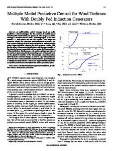
Fig. 2. Sketch of system under consideration. The underlying protocols are abstracted as (random) delays τs (t), τa (t), and loss probabilities pa , ps .
Notice that the solution of the OCP, as well as the closed loop stability, in the sense of asymptotic convergence, are based only on the sampled data measurements x(ti ) at ti ∈ π P , where π P is implicitly determined by defining a proper triggering criterion. How this criterion can be included in the optimization problem is way beyond the scope of this paper, although it represents an interesting open question, since it plays a crucial role in minimizing the network traffic. Moreover, though Theorem 3.1 is in this work applied to NCSs, the obtained results can be used with any asynchronous system for which a proper triggering criterion can be defined (see, for instance, the simulation example in Section V).
Assumption 1: τs (t) ∈ [τs , τs ], τc (t) ∈ [τc , τc ], and τa (t) ∈ [τa , τa ], i.e. delays are random but ultimately bounded.
IV. C ONTROL OVER C OMMUNICATION N ETWORKS When system (1)-(2) is controlled through a communication network, delays, jitters and packet losses can arise — refer to [1], [2], [7], [13], [14] for an overview on NCSs —. In this work, however, we propose an application level solution (see Figure 1) such that the underlying protocol properties can be abstracted as (random) delays and/or probability losses. An illustration of the overall considered system is depicted in Figure 2. In the remainder of the paper τs (t), and τa (t) are used to refer respectively to the measurement and the actuation delays, while computational delays are represented by τc (t). Additionally, it is assumed that information losses in the upand down-link can occur. The corresponding loss probabilities are given by ps (t) and pa (t) respectively. Furthermore, the following assumptions are made:
Assumption 2: δ max + τs + τc + τa < Tp , where δ max is the maximum recalculation interval. Assumption 1 can be relaxed such that longer and unbounded delays can be treated as information losses. A. Delay compensation Temporarily assume that no packet dropout occurs. We can still use the model available at the controller side to compensate the delays by means of the forward prediction ∫ tsi
x(tsi ) =
f (x(t), u(t))dt + x(ti ),
(11)
ti
where tsi = ti + τs (ti ) + τc + τa .
(12)
Notice that to obtain (11), the input for t ∈ [ti ,tsi ) is required to be uniquely known. Therefore, it must be stored in the control buffer to perform the worst case compensation. If the controller’s buffer and the actuator’s buffer coincides, then the state prediction (11) is equal to the real state of the system. When this condition is verified, we say that the input is consistent. Definition (Consistent Input): The applied control input trajectory u(·) is called consistent if u(·) coincides at any time with the input trajectory provided by the controller.
569
WeA16.6 Definition (Input Consistent Control Algorithm): A control algorithm which generates ∀ti ∈ π consistent inputs is called input consistent. The OCP for (11) can be finally solved to obtain the optimal input trajectory u(τ ; x(tsi )), τ ∈ [tsi ,tsi + Tp ).
(13)
u(τ ; x(tsi )), τ ∈ [tsi ,tsi+1 )
(14)
Thus, is dispatched to the actuator with time-stamp tsi . Table I shows the detailed description of the input consistent compensation algorithm. TABLE I Algorithm 1 (EB-MPC with Delays Compensation): ∈ π P;
∀ti t = current global time; Sensor: 1) Measure x(ti ). 2) Send [x(ti )|ts], with ts = ti , to the controller and go to 1. Controller: buffer = [x(ti )|ts]old ; control input = {[u∗ (·)|ts0 ]}; 1) If [x(ti )|ts]new arrives a) If tsnew ≤ tsold , then discard. b) Else buffer = [x(ti )|ts]new . 2) τs = (t − ts), ti = ts. 3) Calculate from u∗ (·; x(ti )) ∈ control input, x(ti + τs (ti ) + τc + τa ).
exists. One needs to prove there exists a proper input sequence which is the same as the one provided in Theorem 3.1 such that both feasibility and convergence follow in a similar way. In the following, ti is used to refer to the system’s relative time. Consider then δ ′ (t) such that δ ′ = δ (t) + τs + τc + τa < Tp . From condition ii) and Algorithm 1, it trivially follows that the corresponding partition π ′ is proper. Define the ith time-stamp of the control trajectory as tsi = ti + τs (ti ) + τc + τs . Consider any tsi for which the OCP admits a solution. By applying the obtained optimal input u∗ (τ ) = u(τ ), τ ∈ [tsi ,tsi+1 ), the state x(tsi+1 ) ∈ X is reached. Moreover, the remaining piece of trajectory u∗ (τ ; x(tsi )) ∈ U, τ ∈ [tsi+1 ,tsi + Tp ), is admissible and leads (4b) to x(tsi + Tp ) ∈ E . According to Algorithm 1 in Table I, the following input is used: { b u (t), for τ ∈ [tsi , tsi+1 ] u(τ ) = , (16) u(τ ), for τ ∈ (tsi+1 , tsi + Tp ] where ub (·) represents the buffered input in the actuator’s buffer. However, according to Algorithm 1, ub (τ ) ≡ u(τ ), for τ ∈ [tsi ,tsi+1 ). Consider ts0 = t0 , then it can be seen from the proof of Theorem 3.1 that (16) coincides with the former input sequence. Eventually, by using the same argumentation, asymptotic convergence to the origin can be proved. B. Information losses compensation So far, only delays were considered. Assume now that the system is also subject to information losses. If this is the case, the state prediction (11) cannot be calculated anymore, since input consistency is not anymore verified. In [15], [16], prediction consistent feedbacks were used to tackle the problem, i.e. feedback trajectories capable of keeping the error between state prediction (11) and actual state small. In this work, instead, we use a different approach based on an acknowledgment mechanism at the actuator side. Though restrictive, the next assumptions are standard practice in NCSs and they are important to re-establish input consistency.
(15)
4) Solve the OCP for (15) −→ u∗ (τ ; x(ti )), for τ ∈ [ti + τs (ti ) + τa + τc ,ti+1 + τs + τa + τc ). 5) Send [u∗ (τ ; x(ti ))|ts], with ts = (t + τa + τc ). 6) Insert [u∗ (τ ; x(ti ))|ts] in control input and go to 1. Actuator: buffer = {[u∗ (·)|ts0 ], . . . , [u∗ (·)|tsn ]}, for ts0 < t < ts1 . . . < tsn ; applied input = [u∗ (·)|ts0 ]; 1) When [u∗ (·)|ts]new arrives a) Insert [u∗ (·)|ts]new in buffer. b) “Sort” buffer by increasing ts. 2) temp = first element of buffer. 3) If tstemp = t a) applied input = temp. b) Remove first element from buffer. 4) Go to 1.
Assumption 3: A mechanism is available such that every piece of information received by the actuator is acknowledged to the controller.
Theorem 4.1 (EB-MPC with Delays Compensation): Consider the closed loop system (1)-(5), subject to the delays τs (t), τc (t), τa (t). If i) There exists an EB-MPC for the system without delays. ii) Assumptions 1 and 2 are verified. iii) System and controller share a common global clock iv) Tp > δ max + τs + τc + τa . v) The algorithm in Table I is used. Then, lim ∥x(t)∥ = 0. t→∞
Proof: The problem that might arise is that due to the presence of nondeterministic delays, the control input trajectory is not defined in between some time interval. It must therefore be shown that a proper input sequence
Assumption 4: The acknowledgments cannot be dropped and they are delivered instantaneously to the controller. With instantaneously delivered we mean here that the acknowledgment delay is negligible. This might for example be guaranteed by a network protocol that allows quality of service and prioritization for specific packets. Despite this, it is possible to relax Assumption 4 allowing dropouts and delays. The compensation algorithm must, however, be modified accordingly to take this phenomenon into account. Nevertheless, notice that to maintain input consistency we must assume that at least one acknowledgment arrives in a finite time. Under Assumptions 3 and 4, we can modify the former algorithm by integrating the acknowledgment mechanism. Thus, if the whole optimal input trajectory
570
WeA16.6
Fig. 3.
Frontal view of the aircraft under control.
(13) is sent to the actuator, it can be used whenever some information is lost. It can be easily deduced that the modified algorithm is input consistent and, under similar conditions, Theorem 4.2 eventually follows. Corollary 4.2 (EB-MPC Under Information Losses): Consider the closed loop system (1)-(5) subject to delays and information losses. If i) There exists an EB-MPC for the system without delays and information losses. ii) System and controller share a common global clock. iii) Assumptions 1-4 are verified. iv) Tp > δ max + j · τs + τc + k · τa < Tp , for j, k ∈ N, with j, k = number of consecutive dropouts respectively in the sensor and actuation channel. v) The modified version of Algorithm 1 is used. vi) u(τ ; x(tsi ), for τ ∈ [tsi ,tsi + Tp ) is dispatched to the actuator. Then, lim ∥x(t)∥ = 0. t→∞
Proof: The proof follows immediately from Theorem 3.1 and 4.1. The use of an input consistent control algorithm guarantees the absence of mismatch between controller and actuation buffer, which allows for feasibility and convergence to be proved similarly to Theorem 4.1. V. S IMULATION R ESULTS In this section a PVTOL aircraft is taken into consideration. The problem is to control the plane depicted in Figure 3 by manipulating the thrust and the roll angular acceleration. The simplified model of the system is represented by the following nonlinear equations: x˙1 (t) = x2 (t) x˙2 (t) = u1 (t − τ1 (t)) sin(θ (t)) y˙1 (t) = y2 (t) , (17) y˙2 (t) = u1 (t − τ1 (t)) cos(θ (t)) − 1 θ˙ (t) = ω (t) ω˙ (t) = u2 (t − τ2 (t))
where x1 (t), x˙1 (t) represent the lateral position and velocity; y1 (t), y˙1 (t) are the vertical position and speed; θ (t), ω (t) are respectively the roll angle and speed. Notice that (17) is not actually a NCS — one could think of a fly-by-wire plane, but this is not necessary the case — but an input delayed system, where the random but bounded delays τ1 (t), τ2 (t) are due to information processing. The objective is to steer the system to the origin by manipulating the thrust, u1 (t), and the roll angular acceleration, u2 (t). The only additional constraint is to avoid that the plane crashes, i.e. y1 (t) ≥ 0. It is assumed that τ1 (t) ∈ [0, 0.3] seconds, and τ2 (t) ∈ [0, 0.4] seconds. We are temporary assuming that no information is lost. Figure 4 shows the comparison between the nominal case (no delays), uncompensated and compensated scenarios. The compensation was done by considering the worst case for both delays, i.e. 0.4 seconds. As one can see, with the proposed algorithm delays are easily counteracted, and the constraints are never violated. On the contrary, without the delay compensation, the plane crashes. Moreover, the obtained qualitatively behavior is comparable to the nominal case. A second simulation was performed to show how the algorithm based on the acknowledgment messages is able to cope with random packet losses. For simplicity no delays are present, although 30% of input trajectories are supposed to be lost. Figure 5 shows how the algorithm suggested in Section IV-B can easily cope with the input information losses and safely steer the system to the origin. VI. C ONCLUSION In this paper, we demonstrated how NMPC can be embedded in a general event-based/asynchronous framework. It can be easily applied also in presence of random delays and information losses, which are, for instance, a common problem in NCSs. In the nominal case, the key requirement to guarantee asymptotic convergence is to choose a sufficiently long prediction horizon. The EB-MPC can be used to considerably reduce both computational requirements and exchanged information by keeping a closed loop behavior comparable to the standard NMPC. A simple but effective algorithm to compensate random measurement, computation and actuation delays was presented. In general, if an input consistent algorithm is available, both delays and information losses, commonly present in control systems, can be easily compensated while maintaining closed loop stability (in the sense of asymptotic convergence). Future work on how to actively schedule the measurements to minimize the information exchange should be done. Similarly, deeper investigation on asymptotic stability and robustness must be investigated. ACKNOWLEDGMENTS The German Research Foundation (DFG) within the scope of the priority research program SPP 1305 is gratefully acknowledged.
571
R EFERENCES [1] J. Hespanha, P. Naghshtabrizi, and Y. Xu, “A survey of recent results in networked control systems,” Proc. of the IEEE, vol. 95, no. 1, pp. 138–162, 2007.
WeA16.6
Fig. 4. Comparison between the nominal case (dashed line), the uncompensated case (dotted line) and the proposed algorithm (solid line), where the compensation was done for the worst case of both delays (0.4 sec.). Notice that without compensation the plane would have crashed.
Fig. 5. Simulation of the system when 30% of the input packets go lost. Again, without compensation, the plane would crash on the ground. On the contrary, the suggested input consistent algorithm can easily counteract the information losses and steer safely the system to the origin.
[2] Y. Tipsuwan and M. Y. Chow, “Control methodologies in networked control systems,” Cont. Eng. Pract., vol. 11, pp. 1099–1111, 2003. [3] R. Brockett and D. Liberzon, “Quantized feedback systems perturbed by white noise,” in Proc. 37th IEEE Conference on Decision and Control, vol. 2, 16–18 Dec. 1998, pp. 1327–1328. [4] W. P. Heemels, J. H. Sandee, and B. P. van den, “Analysis of eventdriven controllers for linear systems,” International Journal of Control, vol. 81, pp. 571–590, 2008. [5] A. Casavola, E. Mosca, and M. Papini, “Predictive teleoperation of constrained dynamic systems via internet-like channels,” IEEE Trans.
Control Syst. Technol., vol. 14, no. 4, pp. 681–694, July 2006. [6] P. L. Tang and C. W. De Silva, “Stability validation of a constrained model predictive networked control system with future input buffering,” International Journal of Control, vol. 80, pp. 1954–1970, 2007. [7] G. Pin and T. Parisini, “Stabilization of networked control systems by nonlinear model predictive control: a set invariance approach,” in Nonlinear Model Predictive Control: Towards New Challenging Applications, ser. Lecture Notes in Control and Information Sciences, L. Magni, D. Raimondo, and F. Allgwer, Eds. Springer, June 2009. [8] L. Gr¨une, J. Pannek, and K. Worthmann, “A networked unconstrained nonlinear mpc scheme,” Submitted to ECC09, Preprint. [9] I. G. Polushin, P. X. Liu, and C.-H. Lung, “On the model-based approach to nonlinear networked control systems,” Automatica, vol. 44, pp. 2409–2414, 2008. [10] F. Fontes, “A general framework to design stabilizing nonlinear model predictive controllers,” Sys. Contr. Lett., vol. 42(2), pp. 127–143, 2001. [11] R. Findeisen, Nonlinear Model Predictive Control: a Sampled-Data Feedback Perspective. VDI Verlag, 2006, vol. 8, no. 1086. [12] D. Q. Mayne, J. B. Rawlings, C. V. Rao, and P. O. M. Scokaert, “Constrained model predictive control: Stability and optimality,” Automatica, vol. 36, no. 6, pp. 789–814, June 2000. [13] D. Quevedo, E. Silva, and G. Goodwin, “Control over unreliable networks affected by packet erasures and variable transmission delays,” IEEE J. Sel. Areas Commun., vol. 26, no. 4, pp. 672–685, 2008. [14] G. Nair, F. Fagnani, S. Zampieri, and R. Evans, “Feedback control under data rate constraints: An overview,” Proc. IEEE, vol. 95, no. 1, pp. 108–137, 2007. [15] R. Findeisen and P. Varutti, “Stabilizing nonlinear predictive control over nondeterministic communication networks,” in Nonlinear Model Predictive Control: Towards New Challenging Applications, ser. Lecture Notes in Control and Information Sciences, L. Magni, D. Raimondo, and F. Allgwer, Eds. Springer, June 2009. [16] P. Varutti and R. Findeisen, “Compensating network delays and information loss by predictive control methods,” in Proc. of the ECC09, 2009, pp. 1722–1727.
572