Evidence for complex, collective dynamics and emergent, distributed computation in plants David Peak*†, Jevin D. West‡, Susanna M. Messinger‡, and Keith A. Mott‡ *Department of Physics, Utah State University, Logan, UT 84322-4415; and ‡Department of Biology, Utah State University, Logan, UT 84322-5305 Communicated by Marlan O. Scully, Texas A&M University, College Station, TX, November 24, 2003 (received for review January 24, 2003)
It has been suggested that some biological processes are equivalent to computation, but quantitative evidence for that view is weak. Plants must solve the problem of adjusting stomatal apertures to allow sufficient CO2 uptake for photosynthesis while preventing excessive water loss. Under some conditions, stomatal apertures become synchronized into patches that exhibit richly complicated dynamics, similar to behaviors found in cellular automata that perform computational tasks. Using sequences of chlorophyll fluorescence images from leaves of Xanthium strumarium L. (cocklebur), we quantified spatial and temporal correlations in stomatal dynamics. Our values are statistically indistinguishable from those of the same correlations found in the dynamics of automata that compute. These results are consistent with the proposition that a plant solves its optimal gas exchange problem through an emergent, distributed computation performed by its leaves.
A
lthough biological and computational systems appear to share many analogous structures and processes (1), rigorous, nontrivial connections between life and computation remain elusive. One difficulty is that the biological systems that have been most actively investigated for evidence of computation (macroscopic organisms with neuronal networks, on the one hand, and proteins and nucleic acids participating in tangled webs of chemical reactions, on the other) are built from elements that interact irreducibly with vast numbers of each other. Such highly interconnected systems are notoriously hard to adequately describe mathematically. Support for the existence of sophisticated computation in biology (if it exists) is probably more likely to be found in systems in which the relevant elements interact sparsely. We propose that plants may be ideal for this purpose. Plants solve a gas exchange problem by using apparatus whose structure is reminiscent of cellular automata (CA), computerbased simulations of locally connected networks (2). Results of experiments we performed involving transient gas exchange and photosynthesis in intact, living leaves are remarkably similar to dynamical behavior observed in some CA that perform specific computational tasks. As we discuss below, these results are consistent with the hypothesis that plants engage in a form of emergent, distributed computation. Our argument is based on ideas drawn, in part, from plant biology and, in part, from computer science and physics. Because most readers will not be conversant with all of these, we first summarize the relevant (and well established) notions from each area. Salient Facts About Plants In bright light, a plant’s stomata [variable aperture pores distributed over its leaves (and other parts) at densities of tens to hundreds per mm2 (Fig. 1a)] tend to open. This creates a dilemma. The plant benefits from the opening because it is able to take in CO2, which it uses in photosynthetic energy storage. At the same time, it also experiences the detriment of increased water evaporation and the consequent risk of water stress. How plants resolve this dilemma has enormously important consequences because, through adjustment of their stomatal apertures, plants are responsible for 99% of terrestrial carbon fixation and 90% of terrestrial water loss. 918 –922 兩 PNAS 兩 January 27, 2004 兩 vol. 101 兩 no. 4
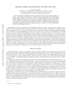
Fig. 1. (a) Confocal micrograph of a 0.56-m2 region of a leaf surface showing a field of (bean-shaped) stomata. (b) Near-infrared image of a 6.25-cm2 region of a leaf surface showing patchy chlorophyll fluorescence. The image is brighter where the leaf’s stomata are more closed.
A central paradigm of plant biology is that, in the face of spatially heterogeneous and temporally varying environmental conditions, a plant continually adjusts stomatal aperture so that, over time, it maximizes CO2 uptake for a fixed amount of water loss (3). The problem is made more difficult because it has to be solved at the level of the entire organism but without the aid of neuronal tissue capable of transmitting signals and coordinating activities over widely separated portions of the plant. Despite decades of intense study, how this is accomplished is not yet completely understood. The aperture of one stoma certainly adjusts to local microenvironmental conditions, and, for many years, stomata have been viewed as a collection of autonomous units responding similarly but independently to environmental conditions. It is now clear that a stoma’s aperture also depends on interactions with neighboring stomata, and that the opening and closing of stomata often become synchronized in spatially extended patches, even under spatially homogeneous environmental conditions (as seen in Fig. 1b, for example). Sometimes, patches have richly complicated dynamics (4). Stomatal patchiness appears to be a ubiquitous feature of plant behavior; it has been observed in ⬎200 species, both in the laboratory and in the field (5). This is somewhat surprising because patchiness supposedly often results in less than maximal CO2 uptake for fixed water loss (6). To date, there is no consensus on the biological function of patchiness or why it is so commonplace. Salient Facts About Cellular Automata That Compute CA are discrete-space, -time, and -state dynamical systems in which the state at any site is determined in the next moment by its own state and those of a small number of neighbors in the current moment. We consider here 1D and 2D CA with spaces of N sites and with boundaries wrapped around in periodic fashion. Each site is at the center of a local neighborhood Abbreviations: CA, cellular automata; SOC, self-organized criticality. †To
whom correspondence should be addressed. E-mail:
[email protected].
© 2004 by The National Academy of Sciences of the USA
www.pnas.org兾cgi兾doi兾10.1073兾pnas.0307811100
Dynamics of Emergent, Distributed Computation Involving Patches Emergent, distributed computation is unlike the standard manipulation of bit strings by logic gates in a PC. How such computation is performed in 1D, 2-state CA has been fully explicated, but the specialized arguments used for that purpose Peak et al.
PNAS 兩 January 27, 2004 兩 vol. 101 兩 no. 4 兩 919
COMPUTER SCIENCES
containing v ⫺ 1 other sites (v ⬍⬍ N), none of which is farther than r from the central site. At any instant, each site is in one of possible states. The state of the site at position xជ at time t ⫹ 1 is given by s(xជ,t ⫹ 1) ⫽ xជ[c(xជ,t)], where c(xជ,t) is the configuration of states at time t of the neighborhood centered on xជ and xជ is a local look-up table that assigns a state to the site at xជ for each of the v possible neighborhood configurations. The combined action of the xជ at each site in every time step implicitly defines a global look-up table, ⌽, that determines how configurations, C(t), of the entire space change from moment to moment: C(t ⫹ 1) ⫽ ⌽[C(t)]. ⌽ assigns a new configuration to the CA space for each of the N possible current configurations. Because ⌽ has vastly more entries than any of the xជ, its properties usually can only be inferred empirically. They are often quite different from the properties of the local xជ and, consequently, are said to be emergent (7). After M successive iterations of ⌽ an ‘‘input’’ configuration, C(0), is transformed into an ‘‘output,’’ C(M). In some instances, such outputs are ‘‘special’’ according to some externally imposed criteria. When this is the case, the action of ⌽ is sometimes interpreted as performing a ‘‘computational task’’ where ‘‘C(M) is the answer to the problem posed by C(0).’’ Performance of the task is both effected by and encoded in the entire space of sites and it is thus distributed over the CA. An especially instructive (and, for our purpose, apt) example of emergent, distributed computation is the density classification task (8). In the density classification task, each site of the CA can be in one of two states: 0 (black) or 1 (white). The ‘‘correct answer,’’ according to one definition of the task, corresponds to the states of all N sites becoming 0 whenever 0 is in the majority in C(0), or all 1 otherwise. If it were possible to simply count the 0s and 1s in the input configuration, determination of the majority state would be trivial; but counting requires some kind of external agent or central processing unit, which a locally connected CA does not possess. How density classification emerges in systems lacking global connectivity has been studied in 1D CA with both uniform (the same xជ at all sites) (9) and nonuniform local rules and, to a lesser extent, in 2D, nonuniform networks (10). Irrespective of dimension or uniformity, a generic feature of density classification is that the local dynamics organizes regions of mixed states into regular patches (regions of all black, all white, or black–white checkerboard patterns) that grow and shrink, and compete with each other for dominance (Fig. 2).
PLANT BIOLOGY
Fig. 2. Space–time diagrams of the 1D GKL classifier CA. The top line in each case has 75 white sites and 74 black sites. (a) ‘‘Easy problem’’ in which the space correctly becomes all white at t ⫽ 140. (b) ‘‘Hard problem’’ created by randomly interchanging the states of two sites in the starting configuration of a. Relaxation to a (wrong, in this case) uniform black state does not occur until t ⫽ 290.
are not directly applicable to the analysis of noisy, 2D, manystate systems, such as stomatal networks. Until effective tools for quantifying computation in such circumstances become available, we will have to be content with drawing tentative inferences from the statistical properties of computational dynamics. Emergent, distributed computation via patch formation is inherently a dynamically unfolding process. There is a qualitative similarity between growing patches of synchronized states in CA that perform density classification and spreading ‘‘avalanches of activity’’ in CA models of self-organized criticality (SOC) (11). (The prototypical SOC system is a CA simulation of a sandpile. In a CA sandpile, the states of the sites are numbers of ‘‘grains.’’ The local rule determines how grains are redistributed from higher to lower neighboring stacks whenever the local height difference exceeds a threshold.) To see whether there is also a quantitative connection, we calculated a number of statistics purported to measure SOC-like, spatiotemporal complexity for (uniform and nonuniform) 1D and (nonuniform) 2D density classifier CA. These measures include the Fourier spectrum (12), Hurst’s rescaled range (R兾S) statistic (13), and event waiting time distribution (14). A barrier to obtaining useful quantities of data for this purpose is the fact that efficient density classifiers rapidly arrive at the correct answer for most initial configurations. Thus, it is necessary to study the computational dynamics of ‘‘hard problems’’ only (those with initial densities close to 0.5 that involve unusually long transient periods). As a specific example, we examined the 1D, uniform, GKL-rule classifier (15), for n ⫽ 149 sites. This CA has v ⫽ 7 (r ⫽ 3) neighborhoods. We generated ⬎1,400 runs, each with a different, randomly selected 75-to-74 initial state distribution, that required at least 160 time steps to settle into a homogeneous state (contrast Fig. 2 a and b). Only a few percent of all configurations with densities near 50% produce such hard problems. The Fourier spectral density for the first 128 time steps of the aggregated time series from these runs was well fit by the power law expression S( f ) ⬀ f⫺PF, where PF ⫽ 1.98 ⫾ 0.02 (R2 ⫽ 0.99; f is frequency). Power law spectral densities are a general feature of SOC systems. Although different SOC systems have different values of PF, sustained avalanche activity in CA simulations of (conservative) sandpiles also yields a spectral density exponent of PF ⫽ 2 (16). Spectral densities that vary as f⫺2 arise whenever the associated signal (for example, average density in the classifier CA or total number of grains in the sandpile CA) changes aperiodically with increments that are small compared with the range of values the signal can take on. The nature and origin of the increments are largely irrelevant. To distinguish whether the increments are a result of uncorrelated, random processes or possibly produced by interesting dynamics, the Hurst R兾S statistic is sometimes used. This statistic attempts to sense long-term regularities in seemingly irregular signals. For our aggregated, classifier time series data we find R兾S ⬀ dH, where H ⫽ 0.82 ⫾ 0.06 (R2 ⫽ 0.94; d is time delay). For comparison, H ⫽ 0.5 for uncorrelated, random increments. For signals with positive long-term correlation (such as is produced by a classifier CA), H ⬎ 0.5. Interestingly, simulations of CA sandpiles also yield H ⫽ 0.8 (17). Finally, we investigated correlations between successive ‘‘events.’’ We defined a classifier ‘‘event’’ to be a change in patch type at a given site. Specifically, we defined an event at a site to be a time series there consisting of 0000 followed by a 1, 1111 followed by a 0, 0101 followed by a 1, or 1010 followed by a 0. Waiting times between successive events at randomly chosen sites followed a frequency distribution of the form FW ⬀ exp(⫺␣W), where ␣ ⫽ 0.032 ⫾ 0.001 (R2 ⫽ 0.99). To interpret the numerical factor, we note that for CA sandpiles, the distribution of waiting times between avalanches of all sizes is supposed to be FW ⬀ exp(⫺W兾具W典) (14). The mean waiting time inferred by identifying the latter expression with our empirical
Fig. 4. Stomatal aperture [or stomatal conductance (SC)], as measured by gas exchange, is inversely correlated with chlorophyll fluorescence [or pixel intensity (PI)]. Data demonstrate that fluorescence is an accurate surrogate for aperture. Fig. 3. State trend images. (Top) A 15 ⫻ 15 sandpile CA. Red sites have more grains than they did six time steps in the past, yellow sites have fewer grains, and black sites have the same number of grains. The activity in the avalanche spreads in a typically irregular fashion. (Middle) A 15 ⫻ 15, nonuniform density classifier CA. Red sites have a higher state value than six time steps in the past, yellow sites have a lower state value, and black sites have the same state value. The activity contains triangular structures that propagate coherently from left to right at constant speed. (Bottom) A 25-mm2 portion of a leaf during dynamical patchiness. Red pixels have a higher fluorescence intensity than they did eight minutes earlier, yellow pixels have a decreased intensity, and black pixels have the same intensity. As in the classifier CA, a coherent, nondispersive (yellow) structure propagates at constant speed (⬇8 m兾s) from the upper left to the lower right.
result, therefore, is 具W典 ⫽ 1兾␣ ⫽ 31.3 ⫾ 1.0, which is statistically indistinguishable from our directly calculated value of 具W典 ⫽ 30.3 ⫾ 0.5. We find similar agreement between SOC dynamics and the dynamics of other 1D and 2D CA performing global computational tasks via patch formation and speculate that this is probably a general result. In sandpile CA, self-organizing avalanches tend to remove large differences in the heights of adjacent grain stacks over spatially extended regions. In classifier CA, self-organizing patch growth tends to remove adjacent state differences over spatially extended regions. This mutual tendency to homogenize spatial differences leads to the similarities in the dynamical statistics noted above. On the other hand, quiescent configurations produced by CA sandpiles and by CA density classifiers are quite different. Sandpile avalanches tend to transform configurations of lower entropy into configurations of higher entropy, whereas patches in classifiers do the opposite. In this sense, sandpile dynamics is diffusive and classifier dynamics is antidiffusive. The difference between these behaviors can be visualized by examining state changes, ⌬s(xជ,t) ⬅ s(xជ,t) ⫺ s(xជ,t ⫺ n). In Fig. 3, ⌬s(xជ,t) ⬎ 0 is coded as red, ⬍ 0 as yellow, and ⫽ 0 as black. Fig. 3 Top shows avalanche activity in a 15-site ⫻ 15-site conservative sandpile, and Fig. 3 Middle shows computational activity in a 15-site ⫻ 15-site, nonuniform, 2D density classifier (M. Sipper, personal communication). The activity in the former is much less organized than in the latter, with changes appearing to be much more unpredictable and with no directed motion. The red and yellow triangular structures in Fig. 3 Middle, on the other hand, traverse the CA space at constant speed. These blocks of information propagate coherently from place to place, much as if they were physical entities, like particles or solitons. As such, they are 2D analogs of the ‘‘particles of information’’ that have been identified as producing computation in 1D CA (9). Experiments (i) Plants solve a formal optimization problem by adjusting the apertures of their stomata. (ii) Stomata are spatially distinct 920 兩 www.pnas.org兾cgi兾doi兾10.1073兾pnas.0307811100
dynamical units that, through local interactions, are capable of forming sparsely connected networks. (iii) Stomata, under some conditions, become synchronized over extended patches. (iv) Solution of a plant’s optimization problem under uniform environmental conditions requires spatial uniformity of stomatal apertures. These points lead us to hypothesize that stomatal networks perform emergent, distributed computation, similar to that found in density classifier CA. As a preliminary test of this hypothesis, we used the results of the previous section and searched for evidence of both SOC-like statistics and the coherent propagation of particles of information in sequences of images of chlorophyll fluorescence obtained from intact leaves of the plant Xanthium strumarium L. (cocklebur). Chlorophyll fluorescence is ideal for this purpose because it can be a spatially explicit indicator of photosynthesis that provides information on several spatial and temporal scales (18, 19). The experimental procedures we used are well established and their details can be found elsewhere (18). The essential points are that the leaves were placed between two separate fan-stirred, temperature-controlled chambers that permitted the passage of light and allowed independent measurement and control of gas mixtures flowing over each surface. Differences in gas composition into and out of the chambers were used to deduce the average stomatal aperture on each leaf surface. The upper leaf surface was illuminated with intense, flat-spectrum light, and the remainder of the plant was in dim illumination. Essentially none of the stomata outside of the illuminated portion of the leaf was open. The gas mixtures in the two chambers were initially identical except that [CO2] in the lower chamber was zero. After leaves reached steady state under these conditions, we initiated dynamics by decreasing [H2O] over the upper surface and maintaining it at the new, reduced value. This perturbation had no effect on stomatal aperture for the lower surface, as measured by gas exchange. Under this condition, observed changes in photosynthesis resulted primarily from changes in the supply of CO2 through the upper surface stomata (20). To quantify these changes, we acquired 8-bit grayscale images (512 ⫻ 512 pixels) of chlorophyll fluorescence from the upper surface by using a sensitive charge-coupled device (CCD) camera. (Light supplied to the leaf was filtered to remove wavelengths ⬎700 nm, while the camera was fitted with a long pass filter that allowed only wavelengths ⬎700 nm.) We recorded images every 20 s for at least 6 h for several different days. The raw data consisted of grayscale movies, some of which can be viewed at http:兾兾bioweb.usu.edu兾kmott兾Complexity㛭Web㛭Page兾complexity㛭homepage.htm. As seen in Fig. 4, there was a strong inverse correlation between average fluorescence intensity per pixel and average aperture per stoma in our experiments. Image pixel density (⬇40,000 pixels per cm2) and actual stomatal surface density (⬇20,000 stomata per cm2) were Peak et al.
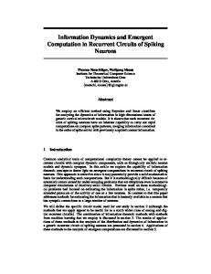
Statistics of Dynamic Stomatal Patchiness Our data consisted of 50,000 intensity time series, each with 512 entries, for randomly selected pixels from three different experimental days. We examined these data for SOC-like correlations. First, the Fourier spectra of the time series were combined and a power law was fit to the resulting spectral density, yielding a best-fit exponent of PF ⫽ 1.72 ⫾ 0.13 (R2 ⫽ 0.65). Our image acquisition system has a noise level of about ⫾3%. This instrumental variability tends to whiten the spectra of our data somewhat at high frequencies and lower the measured value of PF from its true value. Thus, our PF is probably not radically different from that (i.e., 2) of the CA models described previously. Next, the Hurst statistic for our data were fit with a power law yielding a best-fit exponent H ⫽ 0.60 ⫾ 0.03 (R2 ⫽ 0.94). This H, also decreased from its true value by measurement noise, indicates that the collective dynamics manifest in stomatal patches has long-term persistence. Finally, we defined an ‘‘event’’ to be in progress at pixel position xជ at time t if the intensity there was unusually different from what it was n images before: that is, if ⌬I(t) ⫽ 兩I(xជ,t) ⫺ I(xជ,t ⫺ n)兩 ⬍ threshold. We chose n ⫽ 10 as a reasonable compromise between over- and undersampling the dynamics. We found that once such an event had begun, ⌬I typically grew for a while then declined (see Fig. 5, for example). We calculated the waiting time as the interval between the ⌬I maxima for successive events. We found a waiting time distribution for ⬎23,000 events with threshold ⫽ 3 (just above the measurement error) to be well fit by an exponential, FW ⬀ exp(⫺␣W), with 1兾␣ from the fit equal to 6.29 ⫾ 0.40 (R2 ⫽ 0.93). As in our discussion of CA, 1兾␣ may be expected to be a measure of the mean waiting time for SOC-like behavior. Direct calculation of 具W典 from the event data gives 7.88 ⫾ 0.04, a result that is reasonably close to the fit value given that the fit is not for all events. We also calculated event ‘‘size’’ (something we could not do for the density classifier CA examples) as the area under the ⌬I curve for five consecutive Peak et al.
time steps centered on the maximum ⌬I. Event size distribution for SOC-like systems should be a power law, FS ⬀ S⫺PS. Our data, which included ⬎2,000 events of size 24 or greater with threshold ⫽ 7, were well fit by such a form with PS ⫽ 1.77 ⫾ 0.01 (R2 ⫽ 0.99). For comparison, mean field analyses of CA sandpiles (21) yield PS ⫽ 3兾2. Having confirmed that stomatal dynamics is complex in the same way as some CA that perform emergent, distributed computation, we then confronted the issue of the existence of particles of information. Overall, the net response of stomata to lowered humidity is to close, which, in turn, leads to a general increase in fluorescence intensity. Thus, any local decrease in intensity is potential evidence for interesting, nonaverage behavior. Fig. 3 Bottom shows an example sequence of images in which increasing fluorescence intensity is recoded as red and decreasing intensity as yellow. Zero change is black. In that row, blocks of decreasing intensity coherently propagate through a background of increasing intensity. (This is probably because, in changing their aperture, stomata tend to overshoot before settling into a steady condition. Overshooting may be an effective mechanism for sampling aperture state space for ‘‘good answers’’ to a plant’s optimization problem.) The sequence in Fig. 3 is not isolated. We observed similar particle-like behavior in all experiments that had dynamically patchy fluorescence. We infer, therefore, that it is an integral aspect of complex stomatal dynamics. In summary, we have demonstrated that the dynamical properties of stomatal opening and closing on a leaf are essentially identical to those of some CA that perform emergent, distributed computation. Our analyses are only a first step, of course, in connecting computation and plants. If, like CA model systems, leaves really did perform emergent, distributed computation, then the phenomenon of stomatal patchiness would no longer be a puzzle: patchiness is a companion of computation. Moreover, such computation would also be a feat of surprising subtlety. In CA simulations, even though processing occurs without a central controller, a central unit of some kind initiates the computation and later reads out and interprets the ‘‘result.’’ In the case of leaves, stomata are simultaneously the sensors of external information, the processing units that calculate how gas exchange regulation should occur, and the mechanisms for executing the regulation. Thus, in those plants that solve the dilemma of optimal gas exchange, evolution may have found an elegantly parsimonious computational technique in which input, output, and processing are all accomplished by using the same hardware. We thank Eugene Bruce, Tom Buckley, and Graham Farquhar for helpful suggestions, and Rand Hooper for technical assistance. This work was supported by National Science Foundation Grant IBN-0219375. PNAS 兩 January 27, 2004 兩 vol. 101 兩 no. 4 兩 921
COMPUTER SCIENCES
Fig. 5. Waiting-time (squares) and event-size (circles) distributions for fluorescence intensity ‘‘events’’ during stomatal patchiness. (Inset) A small portion of the event data used to determine the distributions.
PLANT BIOLOGY
roughly equal. Thus, it is reasonable to assume that correlations in intensity time series and between pixels arose from similar spatiotemporal correlations in stomatal dynamics. The solution to a plant’s optimization problem is a spatially uniform stomatal aperture, gave(eជ), for every set of spatially uniform environmental input conditions, eជ. Our experiments consisted of recording the details of how the transition, gave(eជ) 3 gave(eជ⬘), resulted from a specific, imposed change eជ 3 eជ⬘. In general, the stomatal response to lowered humidity is to close. Thus, gave(eជ⬘) was always less than gave(eជ) in our experiments. In the vast majority of our experimental runs, we observed that gave decreased monotonically after the applied humidity decrease, reaching its new value in less than an hour. In these cases, fluorescence patches were never observed. Less frequently, gave was observed to oscillate for 1–2 h. These rather brief episodes were always accompanied by at least dim, usually stationary patchiness. On rare occasions, gave oscillated for many hours, and sharply contrasted patches were observed to move about the surface of the leaf in visually complicated ways. A natural interpretation of these observations is that neither the environmental conditions nor the leaf’s aperture configuration are exactly spatially uniform or exactly constant in time, and that the details of how apertures change subsequent to the perturbative lowering of humidity depend sensitively on all of the microscopic variability. The situation is remarkably similar to what is observed in the density classifier simulations. Very small changes in initial state can produce very different dynamical responses. If the analogy between leaf and classifier is apt, then the rare long-transient episodes of dynamic patchiness correspond to particularly hard problems that the leaves struggle to solve. As in our analysis of the dynamics of the GKL classifier, we take advantage of these long episodes for our statistical analyses.
1. Bornholdt, S. (1998) in Non-Standard Computation: Molecular Computing, Cellular Automata, Evolutionary Algorithms, Quantum Computers, eds. Gramss, T., Bornholdt, S., Gross, M., Mitchell, M. & Pellazzari, T. (Wiley, New York), p. 15. 2. Wolfram, S. (1994) Cellular Automata and Complexity (Addison–Wesley, Reading, MA). 3. Cowan, I. R. & Farquhar, G. D. (1977) Symp. Soc. Exp. Biol. 31, 471–505. 4. Cardon, Z. G., Mott, K. A. & Berry, J. A. (1994) Plant Cell Environ. 17, 995–1008. 5. Beyschlag, W. & Eckstein, J. (1998) Prog. Bot. 60, 283–298. 6. Buckley, T. N., Farquhar, G. D. & Mott, K. A. (1999) Oecologia 118, 132–143. 7. Mitchell, M. (1998) in Non-Standard Computation: Molecular Computing, Cellular Automata, Evolutionary Algorithms, Quantum Computers, eds. Gramss, T., Bornholdt, S., Gross, M., Mitchell, M. & Pellazzari, T. (Wiley, New York), p. 95. 8. Packard, N. H. (1988) in Dynamic Patterns in Complex Systems, eds. Kelso, J. A. S., Mandell, A. J. & Schlesinger, M. F. (World Scientific, River Edge, NJ), pp. 293–301. 9. Crutchfield, J. P. & Mitchell, M. (1995) Proc. Natl. Acad. Sci. USA 92, 10742–10746.
922 兩 www.pnas.org兾cgi兾doi兾10.1073兾pnas.0307811100
10. Sipper, M. (1997) Evolution of Cellular Machines (Springer, Berlin). 11. Bak, P., Tang, C. & Wiesenfeld, K. (1987) Phys. Rev. Lett. 59, 381–384. 12. Jensen, H. J. (1998) Self-Organized Criticality (Cambridge Univ. Press, Cambridge, U.K.). 13. Mandelbrot, B. B. & Wallis, J. R. (1968) Water Resourc. Res. 4, 909–918. 14. Sanchez, R., Newman, D. E. & Carreras, B. A. (2002) Phys. Rev. Lett. 88, 1–4. 15. Gacs, P., Kurdyumov, G. L. & Levin, L. A. (1978) Probl. Peredachi Inf. 14, 92–98. 16. Jensen, H. J., Christensen, K. & Fogedby, H. C. (1989) Phys. Rev. B 40, 7425–7427. 17. Carreras, B. A., van Milligen, B., Pedrosa, M. A., Balbı´n, R., Hidalgo, C., Newman, D. E., Sa´nchez, E., Frances, M., Garcı´a-Corte´s, I., Bleuel, J., et al. (1998) Phys. Rev. Lett. 80, 4438–4441. 18. Genty, B. & Meyer, S. (1994) Aust. J. Plant Physiol. 22, 277–284. 19. Siebke, K. & Weis, E. (1995) Planta 196, 155–165. 20. Mott, K. A., Cardon, Z. G. & Berry, J. A. (1993) Plant Cell Environ. 16, 25–34. 21. Lise, S. & Jensen, H. J. (1996) Phys. Rev. Lett. 76, 2326–2329.
Peak et al.