Gait generation for bipedal robots is a very complex problem. ... In the conventional engineering approach, there are two main methods for bipedal gait.
16 Evolution of Biped Locomotion Using Linear Genetic Programming Krister Wolff and Mattias Wahde Department of Applied Mechanics, Chalmers University of Technology Sweden
Open Access Database www.i-techonline.com
1. Introduction Gait generation for bipedal robots is a very complex problem. The basic cycle of a bipedal gait, called a stride, consists of two main phases, namely the single-support phase and the double-support phase, which take place in sequence. During the single-support phase, one foot is in contact with the ground and the other foot is in swing motion, being transferred from back to front position. In the double-support phase, both feet simultaneously touch the ground, and the weight of the robot is shifted from one foot to the other. During the completion of a stride, the stability of the robot changes dynamically, and there is always a risk of tipping over. Thus it is crucial to actively maintain the stability and walking balance of the robot at all times. In the conventional engineering approach, there are two main methods for bipedal gait synthesis: Off-line trajectory generation, and on-line motion planning (Wahde and Pettersson, 2002; Katic and Vukobratovic, 2003). Both these methods rely on the calculation of reference trajectories, such as e.g. trajectories of joint angles, for the robot to follow. An off-line controller assumes that there exists an adequate dynamic model of the robot and its environment, which can be used to derive a body motion that adheres to a stability criterion, such as e.g. the zero-moment point (ZMP) criterion (Li et al., 1992; Huang et al., 2001; Huang and Nakamura, 2005; Hirai et al., 1998; Yamaguchi et al., 1999; Takanishi et al., 1985) that requires the ZMP to stay within an allowable region, namely the convex hull of the support region defined by the feet. An on-line motion controller, on the other hand, uses limited knowledge of the kinematics and dynamics of the robot and its environment (Furusho and Sano, 1990; Fujimoto et al., 1998; Kajita and Tani, 1996; Park and Cho, 2000; Zheng and Shen, 1990). Instead, simplified models are used to describe the relationship between input and output. This method also relies much on real-time feedback information. Control policies based on classical control theory, like the ones outlined above, have been successfully implemented on bipedal robots in a number of cases, see e.g. the references mentioned in the previous paragraph. When the robot is operating in a well-known, structured environment, the abovementioned control methods normally work well. However, the success of these methods relies on the calculation of reference trajectories for the robot to follow. When the robot is moving in a realistic, dynamically changing environment such reference trajectories can rarely be specified, since the events that might occur can never be predicted completely. Furthermore, a control policy based on Source: Climbing & Walking Robots, Towards New Applications, Book edited by Houxiang Zhang, ISBN 978-3-902613-16-5, pp.546, October 2007, Itech Education and Publishing, Vienna, Austria
336
Climbing & Walking Robots, Towards New Applications
conventional control theory will lead to lack of flexibility in an unpredictable environment (Taga, 1994). A shift towards biologically inspired control methods is therefore taking place in the field of robotics research (Katic and Vukobratovic, 2003). Such methods do not, in general, require any reference trajectories (Beer et al., 1997; Bekey, 1996; Quinn and Espenschied, 1993). A common approach in biologically inspired control of walking robots is to use artificial neural networks (ANNs). A review of such methods can be found in (Katic and Vukobratovic, 2003). It is also common to employ the paradigm of artificial evolution (evolutionary algorithms, EAs) to optimize controllers that may consist of, for example, recurrent neural networks (RNNs) (Reil and Massey, 2001), finite state machines (FSMs) (Pettersson et al., 2001), or any other control structure of sufficient degree of flexibility (Boeing et al., 2004). The controller may also consist of a structure coded by hand (Wolff and Nordin, 2001). A related approach is to use genetic programming (GP), which is a special case of EAs, to generate control structures (or programs), for locomotion control of robots, see (Wolff and Nordin, 2003; Ziegler et al., 2002). In some cases, the evolutionary optimization (or generation) of program structures may be applied to a certain component of the overall controller as, for example, in (Ok et al., 2001), where a feedback network was generated using GP. However, to the authors’ knowledge, there exist only a few examples, such as (Wolff and Nordin, 2003; Ziegler et al., 2002), which go beyond parametric optimization and generate also the complete structure of a controller for bipedal walking. As an additional example, in (Wolff et al., 2006), both the structure and the parameters of a central pattern generator (CPG) network were evolved, using a genetic algorithm (GA) as the optimization method. In the work described in this chapter, linear genetic programming (LGP) was used to generate gait control programs from first principles for simulated bipedal robots. Two slightly different approaches will be presented. In the first approach, the control system of the robot consisted of evolved programs generated from a completely random starting point, whereas, in the second approach, the joint torques were forced to vary sinusoidally, even though the (slow) variation of the parameters of the sinusoidal torques was evolved from a random starting point, using LGP. It should be noted that no explicit model of the bipedal system was provided to the controllers in either case, and neither were the evolved controllers given any a priori knowledge on how to walk (except, perhaps, for the forced sinusoidal variation in the second approach).
2. Evolutionary Robotics Many problems in robotics, e.g. the generation of bipedal gaits, can be formulated as optimization problems. Traditional optimization techniques generally require the existence of a mathematical, fixed objective function, i.e. a function f = f ( x1 , x2 , " , xn ) , where
x1 , x2 , " , xn are the variables of the problem. In robotics applications, such as gait generation, the value of the objective function can normally only be obtained by actually letting the robot execute its behavior (for example, walking), and then studying the results. In such applications, even though the value of the objective function can always be obtained, it cannot be computed without an (often lengthy) evaluation of a (physical or simulated) robot. Thus, analytical expressions for, say, the derivative of the objective function cannot be
Evolution of Biped Locomotion Using Linear Genetic Programming
337
obtained. Furthermore, in robotics, the control system (robotic brain) being optimized does not always have a fixed structure. For example, in cases where the robotic control system consists of an ANN, the number of nodes (neurons) in the network may vary during optimization, meaning that the number of variables in the objective function varies as well. Thus, for problems of this kind, other optimization methods than the traditional ones are more appropriate. As the name implies, in evolutionary robotics, the optimization is carried out by means of EAs. In addition to coping with structures of variable size and implicit objective functions of the kind described above, EAs can also handle non-differentiable objective functions containing variables of any kind, e.g. real-valued, integer-valued, Boolean etc. 2.1 Evolutionary Algorithms EAs are methods for search and optimization inspired by Darwinian evolution. An EA maintains a set (population) of candidate solutions to the problem at hand. The members of the set are referred to as individuals. Before the evaluation of an individual, a decoding step is often carried out, during which the genetic material of the individual is used for generating the structure that is to be evaluated. In a standard GA, as well as in certain implementations of GP (such as LGP), the genetic material is in the form of a linear chromosome consisting of a sequence of numbers referred to as genes. After decoding, each individual is evaluated and assigned a fitness value¹ based on its performance. Once the individuals have been evaluated, new individuals are generated by means of genetic operators such as selection, crossover, and mutation. The genetic operators are normally stochastic. For example, selection is normally, and rather obviously, implemented such that individuals with high fitness values have a higher probability of being selected (for reproduction) than individuals with low fitness value. Crossover combines the genetic material of two individuals. Mutations are random modifications of genes that provide the algorithm with new material to work with. 2.2 Linear Genetic Programming LGP is a specific type of EA and, as such, it consists of the same basic components: A population of candidate solutions, the genetic operators, certain selection methods, and a fitness function. The main characteristic of LGP, however, concerns the representation of individuals. An individual in LGP is referred to as a program, and it consists of a linear list of instructions that are executed by a so-called virtual register machine (VRM) during the evaluation of the individual (Huelsbergen, 1996). Common LGP implementations use tworegister and three-register instructions. The three-register instructions work on two source registers and assign the result to a third register, ri := rj + rk . In two-register instructions, the operator either requires only one operand, e.g. ri := sin rj , or the destination register acts as a second operand, e.g. ri := r j + ri (Brameier, 2003). The registers can hold floating point values, and all program input and output is communicated through the registers.
338
Climbing & Walking Robots, Towards New Applications
Fig. 1. Schematic description of the evaluation of an individual in LGP. The input is supplied to the input registers. The constant registers are supplied with values at initialization. During execution by the VRM, the LGP individual manipulates the contents of the calculation registers, by running through the sequence of instructions, starting with the topmost instruction. When the program execution has been completed (i.e. when the evaluation reaches the end of the program), the result is supplied to the output registers Note that the LGP structure facilitates the use of multiple program outputs. By contrast, functional expressions like GP trees calculate one output only. Apart from registers assigned as either input or output registers, a program in LGP consists of registers holding constant values, which do not change during the program execution, as well as registers used as temporary calculation registers. Of course, additional constants can be built during execution, for example by adding or multiplying the contents of two constant registers and placing the results in one of the calculation registers. The values of the input registers are usually protected from being overwritten during the execution of the program. A conceptual description of LGP is given in Fig. 1. In addition to the registers, an LGP instruction consists of an operator. Operations commonly used in LGP are arithmetic operations, exponential functions, trigonometric functions, Boolean operations, and conditional branches (Brameier, 2003). Conditional branching in LGP is usually defined in the following way: If the condition in the IF statement evaluates to true, the next instruction is executed. If, on the other hand, the condition in the IF statement evaluates to false the next instruction is skipped, and program execution jumps to the subsequent instruction instead (i.e. the first instruction after the one that was skipped). The evolutionary search process of LGP begins with a randomly
Evolution of Biped Locomotion Using Linear Genetic Programming
339
generated initial population, and is driven by the genetic operators selection, crossover and mutation. Selection favors individuals with high fitness values.
Fig. 2. Two-point crossover in LGP. Two crossover points are randomly chosen in each parent’s genome. The instructions between the crossover points are swapped, and the resulting individuals constitute the offspring Any of the fitness-proportionate selection schemes commonly associated with EAs, or tournament selection, may be applied with LGP. Crossover works by swapping linear genome segments of parent individuals as shown in Fig. 2. The mutation operator simply replaces a randomly chosen instruction by another, randomly generated, instruction. Finally, as in any application involving an EA to search for a sufficiently good solution in a complex problem domain, finding a proper fitness measure that guides the evolution in the desired direction is crucial. This issue will be further discussed in Subsects. 3.1.4 and 3.2.4.
2.3 Evolution in Physical Robots Versus Simulations In the work described in this chapter, evolution of robot controllers has been studied using realistic, physical simulators. Furthermore, in previous work, as well as in the work of other
340
Climbing & Walking Robots, Towards New Applications
researchers, evolution of gait programs in real, physical robots has been investigated as well (Wolff and Nordin, 2001; Wolff et al., 2007; Ziegler et al., 2002). As clearly shown by those examples, evolution in real, physical hardware is indeed achievable. In general, however, evolution in hardware is much more challenging than evolution in simulators, for several reasons: First, evolution in real robots can be very demanding for the hardware (i.e. the robots), thus requiring frequent replacement of parts such as servo motors. Obviously, this problem does not occur in simulations. Second, the process of evolution in a simulator can relatively easily be parallelized, given that appropriate computational resources are available. A straightforward approach for parallelization is to divide the population into a number of subpopulations, or demes, where each deme is assigned to a separate processor. In such applications, individuals are allowed to migrate (with low probability) from one deme to another during evolution. A corresponding parallelization in the case of evolution in real, physical robots would be more difficult and costly: It would require multiple instances of the robot, as well as duplicate experimental environments. However, there are some examples of an ER methodology, where the entire evolutionary process takes place on a population of physical robots (Ficici et al., 1999; Watson et al., 1999). Third, evaluation of individuals in simulators can often be carried out several times faster than real-time, which is not the case for evaluation of individuals in real robots: Evolution in physical robots is very time-consuming, something that normally restricts the number of evaluated generations considerably (Wolff and Nordin, 2001; Wolff et al., 2007). While evolution in simulators is more convenient from the researcher’s viewpoint than evolution in physical robots, the simulation approach presents other problems. The main issue concerns whether the controllers obtained from the simulation can be transferred to a real, physical robot. This problem is referred to as the reality gap (Jakobi et al., 1995). Although there are some serious difficulties associated with the process of transferring evolved programs to a real, physical robot, for the type of study presented here there is no realistic alternative to simulations: Evolution of bipedal gait controllers, in the way described in this chapter, could hardly be achieved directly in a real, physical robot, due to the large number of evaluations required in order to obtain useful results. Furthermore, regardless of the difficulties involved in transferring simulations results to physical robots, a simulation study may provide valuable qualitative insight concerning, for example, the choice of suitable sensory modalities, before the (often costly) construction of a physical robot is initiated.
3. LGP for Bipedal Gait Generation While LGP can, in principle, be applied to almost any optimization problem, some adjustments and special considerations are of course needed in complex applications such as gait generation. In the work described here, two different implementations of LGP were used, namely (1) an implementation in the C language using the Open Dynamics Engine1 (ODE) physics simulator, and (2) an implementation using the EvoDyn physics simulator (Pettersson, 2003). In the following subsections these two implementations will be described in detail. 1
http://ode.org/
Evolution of Biped Locomotion Using Linear Genetic Programming
341
Fig. 3. The leftmost panel shows the bipedal model used in the ODE simulations, and the second panel from the left shows its kinematics structure with 26 DOFs. The two right panels show the 14-DOF robot model used in the EvoDyn simulations
3.1 ODE Implementation 3.1.1 Physics Simulator In the first implementation the ODE simulator was used. This simulator is available both for the Windows and Linux platforms. In ODE, the equations of motion are derived from a Lagrange multiplier velocity-based model, and a first order integrator is employed. The bipedal model used in connection with ODE has 26 degrees of freedom (DOFs) and is shown in the two leftmost panels of Fig. 3. 3.1.2 Controller Model In the ODE implementation, a motor is associated with each joint. The physics engine is implemented in such a way that the motors can be controlled by simply setting a desired speed and a maximum torque that the motor will use to achieve that speed. However, in this implementation the speed and maximum torque values of each joint motor were preset. Thus, the evolving controller just has to set the rotational direction, (+) or (ï), for each joint of the robot. The control loop as a whole is executed in the following way: (the numbers below correspond to the numbers shown in Fig. 4) (1) At time step t the robot’s sensors receive perceptual input S, which is fed into the sensor registers. Simultaneously, the robot’s current joint angles are recorded in both the input and output (I/O) registers, and in the calculation registers (the constant registers were supplied with values at the LGP initialization). (2) The VRM then executes the program specified by the LGP-individual, manipulating the contents of the calculation registers. During this stage, the I/O, sensor, and constant registers are read-only. (3) When program execution has been completed (i.e. when the last instruction of the program has been executed), motor signal generation (MSG) is initiated: A modified signum function, defined as
− 1 if x < k ° ε ( x) = ®+ 1 if x > k ° 0 otherwise ¯
(1)
342
Climbing & Walking Robots, Towards New Applications
Fig. 4. Schematic depiction of the flow of information through the robot control system, which consists of the following main parts: The LGP-individual, which specifies the control program, the VRM, which interprets and executes the LGP individual, the MSG module, which generates the actual motor signals, and the registers, which constitute the interface between the control system and the robot is then applied to the contents of the calculation registers, and the result is placed in the I/O registers. The value of the parameter ț was empirically determined to 0.12, and this value was used throughout the simulations. (4) These motor signals are then sent to the robot for execution in time step t + K . Thus, motor signals are only updated every K th time step, in order to avoid very rapid (and therefore unrealistic) oscillations of the joints. 3.1.3 Simulation Setup The ODE implementation was used in 60 independent simulation runs, in which the effects of varying specific parameter settings were examined, as illustrated in Table 3. In these simulations the robot was controlled by a program specified by an LGP-individual, as described in the previous subsection. Current joint angles were used as input to the controller, together with measurements, obtained directly from the physics simulation, of linear and angular accelerations of certain body parts of the robot. The registers used by the VRM were implemented in the following way: Registers r1 − r26 were used as input and output registers, i.e. they were fed with the robot’s current joint angle positions in the input stage of the control loop, and then fed with motor signals in the
Evolution of Biped Locomotion Using Linear Genetic Programming
343
Table 1. Instruction set used in the simulations output stage. There was one register of this type associated with each DOF of the robot. The registers r27 − r52 were assigned as internal calculation registers of the VRM, i.e. they could be used to store intermediate results of the computations. At the beginning of the LGP run, registers r53 − r55 were supplied with constant values, and finally, registers r56 − r67 were associated with sensor input. The sensor signals used were the linear acceleration rates of the robot’s feet in three dimensions, and the linear and angular acceleration rates of the robot’s head, also in all three dimensions. A first-order, moving average filter with a window size of ten time steps was used with the sensor signals. In this implementation an instruction was encoded as a set of integers, e.g. {55, 51, 3, 42}. The first and second elements of an instruction refer to the registers to be used as arguments, the third element corresponds to the operator, and the last element determines where to put the result of the operation. The complete instruction set is shown in Table 1. The arithmetic operators used here were encoded in the chromosome as add = 1, sub = 2, mul = 3, div = 4, and sine = 5. Conditional branching operators were encoded in the third element as 6 = if ( r [ j ] > r [k ]) ,
and 7 = if ( r [ j ] ≤ r [k ]) . When decoded, the instruction given above as an exmple is interpreted as r[42] = r[55] × r[51]. Furthermore, in order to avoid division by zero, a slightly modified division operator was defined such that, if the denominator was exactly equal to zero, the operator returned a large, but finite, constant value, here set to 108 . In the simulations, all individuals started from the same upright pose, oriented with their sagittal plane parallel to the x-axis. All the individuals were evaluated for a time period of 36 seconds, long enough for the robot to have the possibility of completing several gait cycles. There were several ways in which the evaluation process of an individual could be terminated: First of all, there was, as already mentioned, a maximum allowed evaluation time for every individual. Second, if an individual caused the robot to fall over before its maximum evaluation time was reached, the evaluation was automatically terminated. Third, excessive energy consumption, as described below, could also cause the termination of an individual. Last, in order to speed up the evolutionary process, another conditional termination criterion was introduced, defined according to the following expression:
344
Climbing & Walking Robots, Towards New Applications
F (i ) + ic Fc + ic < ti ic
(2)
Table 2. Parameters used in the ODE-based simulations where F (i ) equals the fitness contribution at time step ti , Fc and ic are constants, set to 20.0 and 1000 respectively. The interpretation of the above inequality is that the fitness contribution in each time step should grow at least linearly with time. The right hand side of the inequality is a constant, specifying the minimal growth rate accepted. If the expression evaluates to true at some point, evaluation of that individual is terminated immediately. Thus, with this termination criterion, individuals that spent most of their evaluation time standing idle were terminated more quickly than would otherwise have been the case, resulting in a significant saving of simulation time. In addition, such individuals automatically received a lower fitness value, as a result of the premature termination. Furthermore, in order to favor the emergence of human-like gaits, an energy discharging function was included in the simulations. It was motivated by the fact that human bipedal locomotion is very energy efficient, compared with the gaits of humanoid robots. For instance, the state-of-the-art Honda humanoid Asimo uses at least 10 times the energy (scaled) of a typical human when walking (Collins et al., 2005). Each individual was allowed only to use a specific amount of energy as it moved. In general, the work performed by a (generalized) force in circular motion, moving from an angle ϕ a to ϕ b , is defined as ϕb
Wba =
³ Μ dϕ
(3)
ϕa
where Μ is the applied torque. The energy consumption E jt of the j th joint during time step t equals the work performed by that joint during the time step. In the simulations, time was discrete, and the applied torque was constant during each time step. Thus, the total energy consumption is given by:
Evolution of Biped Locomotion Using Linear Genetic Programming
Etot = ¦ E jt = ¦(ϕ b , jt − ϕ a , jt ) Μ ba , jt j ,t
345 (4)
j ,t
When the total energy consumption Etot reached some predefined value, evaluation of that individual was terminated. 3.1.4 Optimization Procedure The optimization was carried out using a steady-state EA with tournament selection. The tournament size was set to four. Furthermore, two-point crossover and mutation, as described in Subsect. 2.2, and in (Brameier, 2003), were implemented. In the 60 independent simulation runs performed, specific parameter values were examined according to Table 3. In order to guide the evolution towards human-like gaits, much time was spent on finding an appropriate fitness function. First, in a previous study by (Wolff and Nordin, 2003) it was
Table 3. Parameters examined in connection with the ODE-based simulations assumed that including a term in the fitness function measuring the height of the robot’s center of mass above the ground should be important. However, it was found that such a term did not improve the results: The robot was instead prevented from moving freely enough to improve its gait. Consequently, that term was simply skipped. Second, another problem arose when the evolved gait controllers had reached a level of performance where they could balance the robot in an upright standing pose. In order to reach higher levels of fitness they just let the robot stand idle almost until the end of the evaluation time, and then the robot took a large leap forward. By doing so, the controllers obtained a reward for distance covered over the trial, and the fact that the robot would have fallen to the ground, had the evaluation time been slightly longer, did not affect the fitness negatively. Finally, a good fitness measure was found to be the following: N
F = ¦ ( xR + xL )
(5)
t =1
where N is the number of time steps in the simulation and x R and x L are the position coordinates of the robot’s right and left foot, respectively, in its initial direction of heading, along the x-axis. The motivation for this fitness measure is that it gives a small reward in
346
Climbing & Walking Robots, Towards New Applications
each time step. Thus, with this measure, individuals that remain idle for a large part of the evaluation time receive lower fitness. Thus, for a given distance covered, this fitness measure favors a gradual movement, rather than a quick leap towards the end of the simulation time. 3.2 EvoDyn Implementation As mentioned earlier, in the ODE implementation described above, the user sets target speeds rather than joint torques. In order to make it possible to explicitly specify a more natural (sinusoidal) variation in the control torques, a different implementation was tried as well. In this implementation, the EvoDyn simulation library, developed at Chalmers University of Technology, was used (Pettersson, 2003). 3.2.1 Physics Simulator Implemented in object-oriented Pascal, EvoDyn is capable of simulating tree-structured rigid-body systems and runs on both the Windows and Linux platforms. Its dynamics engine is based on a recursively formulated algorithm that scales linearly with the number of rigid bodies in the system (Featherstone, 1987). For numerical integration of the state derivatives of the simulated system, a fourth order Runge-Kutta method is used. Visualization is achieved using the OpenGL library2. A fully three-dimensional bipedal robot with 14 DOFs, shown in the two rightmost panels of Fig. 3, was used in the simulations. 3.2.2 Controller model In EvoDyn, torques are applied directly to each joint. In the EvoDyn-based simulations, the torque on joint i varied according to
ri (t ) = Ai sin( k i t + δ i ), i = 1, ! , 14.
(6)
where, in turn, the values of the parameters Ai , k i and δ i were allowed to vary slowly, the rate of variation being determined by the output from a VRM. Letting arbitrary parameter ( Ai , k i or δ i ) the variation was taken as
dz = c tanh r dt
z
denote an
(7)
where c is a constant and r an output register from the VRM, corresponding to the parameter in question. The tanh function was introduced in order to limit the rate of variation to the interval [− c, c ] . Thus, even in cases where the contents of the output registers varied strongly between time steps, the variation in the corresponding parameter would be more gentle than in the ODE implementation described above, provided, of course, that the value of c was sufficiently small. 2
http://opengl.org
Evolution of Biped Locomotion Using Linear Genetic Programming
347
In the EvoDyn implementation, the perceptual input consisted of (1) current joint angles for the 14 joints, and (2) readings from eight touch sensors (four under each foot), filtered using a moving average with a window size of 25 time steps. The time step length was 0.002 s, and the maximum simulation time was set to 20 s. The control loop for the simulation was quite similar to the one used in the ODE implementation: Every K th time step, the perceptual input was measured, and stored in the sensor registers (see the next subsection for a description of the registers) of the VRM. Next, the VRM executed the program specified by the LGP-individual, thus modifying the contents of the calculation registers. The contents of the output registers were then used for computing the variation of the parameters Ai , k i and δ i , as described above. Finally, the torques were applied to the robot’s joints. The interval (number of time steps) K between successive updates was set to 25. Between updates, the applied torques were constant. 3.2.3 Simulation Setup In the EvoDyn implementation, a hybrid evolutionary algorithm was used, in which the genome of the individual consisted of two chromosomes: one that specified the sequence of instructions executed by the VRM (i.e. the LGP-individual, using the same nomenclature as for the ODE-based simulations), and one that set the initial values (for the individual in question) of the 42 parameters Ai , k i , and δ i as well as the 42 parameters (c, in Eq. (7)) determining the rate of variation of Ai , k i , and δ i . Thus, the second chromosome was used as in a standard genetic algorithm, i.e. essentially as a lookup-table. Compared to the ODE implementation, a slightly different specification of registers (for the VRM) was used: Registers r1 − r14 were used as input registers, storing the joint angles. In addition, registers r63 − r70 were used for storing the (filtered) readings from the eight contact sensors under the feet. Registers r15 ï r59 were used as calculation registers, whereas registers r60 − r62 were used for storing the constant values 0.1, 0.01, and 0.001, respectively. Registers r15 − r59 were initialized to zero before each execution of the LGP-individual. Once every K th time step, when the execution of the LGP-individual had been completed, the contents of registers r15 − r28 were used as output determining the variation in the parameters Ai , as in Eq. (7). Similarly, the contents of registers r29 − r42 and r43 − r56 were used for determining the variation of ki and δ i , respectively. The instruction set was the same as for the ODE implementation, see Table 1. As in the ODE implementation, a combination of termination criteria was used during the evaluation of individuals. Simulations were terminated if either (1) the maximum simulation time was reached, (2) the center-of-mass of the robot dropped below a prespecified threshold (indicating that the robot had fallen over), or (3) the center-of-mass of the upper body dropped below that of the waist, indicating that the robot was attempting to use the upper body as a third leg. In some runs, additional termination criteria were added. For example, simulations could be terminated if the robot deviated strongly from a straightline path or if it took a very long initial step (in which case it would gain an immediate fitness increase, but would then find it difficult to retain its balance).
348
Climbing & Walking Robots, Towards New Applications
3.2.4 Optimization Procedure In the EvoDyn-based simulations, an EA with population size P was used. Tournament selection was used, again with each tournament again involving four individuals. However, in the EvoDyn-based simulations, generational replacement was used instead of steady-state replacement. For the first chromosome (specifying the program executed by the VRM), twopoint crossover was used whereas, for the second chromosome, a single crossover point was used. Several different fitness functions were tried, following essentially the sequence described in Subsect. 3.1.4 above. In the end, the fitness measure was taken as in Eq. (5), but with a punishment for sideways deviation, i.e. N
F = ¦ ( x R + x L − y R − y R0 − y L − y L0
(8)
t =1
where y R0 and y L0 denote the initial y-coordinates of the feet.
4. Results In this section the results obtained with the two different implementations will be presented, starting with the results from the ODE-based simulations. 4.1 Results from the ODE implementation The parameter values examined in the ODE-based simulations are shown in Table 4, and the simulation results are summarized in Table 5. The parameters were varied, one at a time, 5
from their default values, resulting in 20 unique parameter combinations (thus, not all 4 possible parameter combinations were tested). In order to increase the reliability of the results, each parameter setting was evaluated in three separate runs. In Table 5, max ( f max ) denotes the best fitness value obtained in any of the three separate runs for the parameter setting in question, f max denotes the average of the best fitness values obtained in the three runs and s ( f max ) denotes the standard deviation. Finally, f avg denotes the average (over the three runs) of the average fitness values (taken over the population).
Table 4. The different parameter settings examined in the ODE-based simulations. The default values are typeset in italic
349
Evolution of Biped Locomotion Using Linear Genetic Programming
The
best
overall
fitness
values
were
obtained
for
the
parameter
settings
P = 128, Li = 128, pc = 0.8, rmut = 0.2, and Ei = 256 and Ei = 256 . As is clear from Table 5, the default parameter values of P and rmut produced the best fitness values. The (default) value of 0.8 for the parameter pc also gave the best result, at least in terms of the f max and f avg fitness values. On the contrary, when considering only the best fitness value of a single individual, a
pc
value of 0.0 (i.e. only mutation used) gave better results, albeit with a large
standard deviation. For
Li
and Ei , the best values turned out to be 32 and 256,
respectively. It should be noted that, with a few exceptions, the difference in performance between the various parameter settings is not statistically significant. The best individual found had a fitness value of 8958. During its 36 s evaluation time (4000 time steps), the robot covered a distance of 1.93 m. The graphs of Fig. 6 show covered distances, d (t ) , for the best individual found and for two other individuals, for comparison. As is clear from the figure, the best individual (i.e. the one labeled ’8958’) moved the longest distance during the evaluation time. At the end of the evaluation period, however, it fell backwards, an event indicated by the drop in the graph of d (t ) at the end. The other two individuals both remained on their feet for the whole evaluation period, but they received lower fitness values. The cyclic nature of the robots’ movements can be seen as oscillations in the curves shown in the figure.
Table 5. Results from the parameter study using the ODE implementation. The first column shows the fitness values of the best individual, max ( f max ) obtained for each parameter setting; The second and third columns show the averages, f max , over the three runs (for each parameter setting) of the best fitness values as well as the standard deviations s ( f max ) (over the three runs) of the same values; The fourth
350
Climbing & Walking Robots, Towards New Applications
column shows the average f avg (over the three runs) of the average fitness values in the population. All values were measured after 25000 selection steps (tournaments). Each of the five partitions of the table shows the variations of a single parameter value. Numbers in bold represent the best fitness values of each partition 4.2 Results from the EvoDyn implementation As will be further discussed below, the gaits obtained using the ODE implementation were, in fact, not very human-like. In order to try to overcome this problem, the EvoDyn implementation, allowing direct sinusoidal variation in the control torques, was tested. Several runs were carried out, using population sizes (P) in the range [30, 500], and initial lengths of the LGP programs (obtained from the first chromosome, as described in Subsect. 3.2) in the range [8, 512]. In most runs, the best evolved controller managed to keep the robot upright for the duration of the simulation (20 s, corresponding to 10000 time steps). Furthermore, the robots normally managed to take one or a few human-like steps forward, as can be seen in Fig. 7. However, continuous human-like walking was not achieved: After the first few steps, the robot normally got stuck with the back foot seemingly glued to the ground. However, in a few rare cases
Fig. 5. Top panel: Walking scene of the bipedal robot in the ODE-based simulations. Starting from the left, the double support phase is depicted (a), followed by the single support phase with the left foot in swing motion (b). Then another double support phase is shown (c), followed by single support phase with the right foot in swing motion (d). Finally, the gait cycle is completed with a double support phase (e). Bottom panel: Plot of the depicted gait cycle. The graphs show the height above ground, h(t ) , of the center-of-mass of the left foot (solid line) and the right foot (dashed line), respectively. The vertical lines indicate the double- and single support phases (a) through (e)
Evolution of Biped Locomotion Using Linear Genetic Programming
351
the evolved robots would walk essentially as in the ODE implementation, taking very short steps. An example of such a case is shown in Fig. 8. Here, the length of the first step was roughly equal to the length of the foot. The robot then moved the back foot in line with the front foot. All subsequent steps were significantly shorter, as indicated by the two rightmost panels of the figure. Note the somewhat peculiar, backwards-leaning posture of the robot.
5. Discussion and Conclusion This study has been centered on essentially model-free evolution of bipedal gaits, in which the controller was not provided with any model of the bipedal robot, neither any a priori knowledge on how to walk. In both the ODE and EvoDyn implementations, the gaitgenerating controller programs were evolved starting from random sequences of basic LGP instructions (supplemented by initial values of the parameters used for specifying the torques, in the EvoDyn case).
Fig. 6. Graphs of covered distances in the ODE-based simulations, d (t ) , during 4000 evaluation time steps, for three different individuals. These individuals received fitness scores of 8958, 5728 and 5591, respectively. The individual with fitness value 8958 was actually the best individual found in any run With the ODE implementation, evolution generated individuals that made the simulated robot walk forward almost indefinitely, albeit very slowly. In fact, some of the best individuals were actually capable of producing locomotion behavior lasting more than thirty times the evaluation time used during evolution. For example, the individual labeled ’5592’ was capable of keeping the robot upright and (slowly) walking for at least 20 minutes. However, no individuals obtained with the ODE implementation reached a walking speed exceeding 0.054 m/s. Considering the fact that the dimensions of the simulated robot were similar to those of a (small) human being, this is indeed a very low walking speed. Even the best individuals made the robot lift its feet only a small distance above the ground while walking, and the step length was also very small (see Fig. 5). As a result, the walking speed of the robot was very low. It appears that these individuals had difficulties in activating the knee joints very much, instead relying on the hip joints, making each step quite short.
352
Climbing & Walking Robots, Towards New Applications
A possible reason for these somewhat discouraging results may be derived from the manner in which joint torques (or set speeds, in the ODE case) were generated: Every K th time step of a simulation, the robot must execute its LGP program, generating torque values based on current sensor readings. While an LGP program can, in principle, provide any form of variation in the registers of the VRM, it is rather unlikely to find, in a huge search space, the kind of smooth, cyclic variation generally associated with bipedal locomotion. This realization prompted the use of the second (EvoDyn) implementation, which allows direct setting of the control torques. Here, a slightly different approach was used, in which sinusoidally varying torques were applied, and the LGP program was used for determining the rate of variation of the parameters specifying the sinusoidal torques. With this implementation, the evolved individuals did indeed take larger steps or, rather, one large step. After the first step (or, in rare cases, a few steps), the evolved robots generally had difficulties proceeding: Either they simply fell over, or (more commonly) they stopped, incapable of moving the back foot forward. The obvious way of avoiding large initial steps is to alter the fitness measure so that large steps are discouraged, for example by reducing the fitness if the distance (in the x-direction) between the two feet exceeds a certain
Fig. 7. The left panel shows the initial posture used in the EvoDyn-based simulations. The two panels on the right show typical first steps taken by evolved individuals. As can be seen, the first step was commonly quite long, making it difficult for the robot to maintain its posture in subsequent steps
Fig. 8. An example of a successful gait obtained with the EvoDyn implementation. With the exception of the first two steps, the robot moved by taking very small steps
Evolution of Biped Locomotion Using Linear Genetic Programming
353
threshold. This approach was indeed tried and while the step length was reduced, the modification instead generated other unwanted behaviors. For example, many individuals started walking on their toes, much like a ballet dancer (but, alas, with much less skill), in order to minimize the distance between the feet in the direction of motion. Further modifications of the fitness measure, intended to remove also these adverse effects, only caused other problems to emerge. These problems are indicative of a more general difficulty commonly present in the evolution of bipedal gaits, namely the problem of specifying a good fitness measure. As mentioned above, a significant effort was made in order to find the best possible fitness measure. Naive candidates generally give poor results. For example, if the fitness measure is taken as the distance walked (measured, for instance, by the position of the robot’s centerof-mass), the robot will simply throw its body forward. Attempts at modifying the fitness measure to avoid such behaviors normally create more problems than they solve: There is always some loophole that evolution can use in order to obtain high fitness values without, at the same time, walking properly. These problems, of course, stem from the difficulty of going from a more or less random starting point to a state of walking: Even though humanlike, continuous walking would generate higher fitness values than any of the behaviors that actually emerge, finding such a solution in the gigantic search space of all possible ways of specifying joint torques is very difficult indeed. In the end, essentially the same fitness measures were used in both implementations (with an added punishment for sideways deviation in the EvoDyn case), see Eq. (8). By integrating the positions of the feet (in the direction of motion) this fitness measure allows the ODE implementation to generate careful, slow steps. The EvoDyn implementation, being forced to apply sinusoidal torque variations, had more difficulties in generating such gaits, even though they did appear in rare cases. A further explanation for the somewhat poor results with respect to gait quality obtained in the simulations presented here compared, for example, to the results obtained in (Wolff et al., 2006), could be the choice of sensor feedback: In the implementations used here, the feedback consisted of joint angles supplemented by a balancing sense (in the ODE case) or touch sensors in the feet (in the EvoDyn case). However, unlike the simulations in (Wolff et al., 2006), which were based on a more elaborate structure involving central pattern generators (CPGs), the feedback did not include the angles of the waist, thigh, and leg relative to the vertical axis. Apparently, this feedback seems to be more important (and perhaps also easier for the controller to interpret and use) than the feedback signals used in the study presented here. A thorough investigation of this issue is a topic for future work. On the other hand, it is known that tactile feedback from the foot, indicating foot-to-ground contact, is essential for human locomotion (Van Wezel et al., 1997). To summarize, the current study has shown that entirely model-free evolution of bipedal gaits (as in the ODE case) is indeed feasible, but that the generated gaits, while stable, are unlikely to be very human-like.
6. Acknowledgment The authors wish to thank Dr. Jimmy Pettersson for providing the EvoDyn simulation library, and Mr. David Sandberg for valuable comments on the manuscript.
354
Climbing & Walking Robots, Towards New Applications
7. References Beer, R. D., Quinn, R. D., Chiel, H. J., and Ritzmann, R. E. Biologically inspired approaches to robotics: What can we learn from insects? Communications of the ACM, 40(3):30– 38, 1997. Bekey, G. A. Biologically inspired control of autonomous robots. Robotics and Autonomous Systems, 18(1–2):21–31, 1996. Boeing, A., Hanham, S., and Bräunl, T. Evolving autonomous biped control from simulation to reality. In Proceedings of the Second International Conference on Autonomous Robots and Agents, pages 440–445, Palmerston North, New Zealand, 2004. Brameier, M. On Linear Genetic Programming. PhD thesis, Dortmund University, Dortmund, Germany, 2003. Collins, S. H., Ruina, A. L., Tedrake, R., and Wisse, M. Efficient bipedal robots based on passive-dynamic walkers. Science, 307:1082–1085, 2005. Featherstone, R. Robot Dynamics Algorithms. Kluwer Academic Publishers, 1987. Ficici, S., Watson, R., and Pollack, J. Embodied evolution: A response to challenges in evolutionary robotics. In Proceedings of the Eighth European Workshop on Learning Robots, pages 14–22, Lausanne, Switzerland, 1999. Fujimoto, Y., Obata, S., and Kawamura, A. Robust biped walking with active interaction control between foot and ground. In Proceedings of the International Conference on Robotics and Automation, volume 3, pages 2030–2035, Leuven, Belgium, 1998. Furusho, J. and Sano, A. Sensor-based control of a nine-link biped. International Journal of Robotics Research, 9(2), 1990. Hirai, K., Hirose, M., Haikawa, Y., and Takenaka, T. The development of Honda humanoid robot. In Proceedings of the International Conference on Robotics and Automation, volume 2, pages 1321–1326, 1998. Huang, Q. and Nakamura, Y. Sensory reflex control for humanoid walking. IEEE Transactions on Robotics and Automation, 21(5):977–984, 2005. Huang, Q., Nakamura, Y., and Inamura, T. Humanoids walk with feedforward dynamic pattern and feedback sensory reflection. In Proceedings of the International Conference on Robotics and Automation, pages 4220–4225, 2001. Huelsbergen, L. Toward simulated evolution of machine–language iteration. In Proceedings of the First Annual Conference on Genetic Programming, pages 315–320, Stanford University, CA, USA, 1996. Jakobi, N., Husbands, P., and Harvey, I. Noise and the reality gap: The use of simulation in evolutionary robotics. In Advances in Artificial Life: 3rd European Conference on Artificial Life, LNCS 929, pages 704–720. Springer, 1995. Kajita, S. and Tani, K. Adaptive gait control of a biped robot based on realtime sensing of the ground profile. In Proceedings of the International Conference on Robotics and Automation, pages 570–577, 1996. Katic, D. and Vukobratovic, M. Survey of intelligent control techniques for humanoid robots. Intelligent and Robotic Systems, 37(2):117–141, 2003. Li, Q., Takanishi, A., and Kato, I. Learning control of compensative trunk motion for biped walking robot based on ZMP stability criterion. In Proceedings of the 1992 IEEE/RSJ International Conference on Intelligent Robots and Systems, pages 597–603, Raleigh, NC, USA, 1992.
Evolution of Biped Locomotion Using Linear Genetic Programming
355
Ok, S., Miyashita, K., and Hase, K. Evolving bipedal locomotion with genetic programming —a preliminary report—. In Proceedings of the Congress on Evolutionary Computation, CEC’01, pages 1025–1032, Seoul, South Korea, 2001. Park, J. and Cho, H. An on-line trajectory modifier for the base link of biped robots to enhance locomotion stability. In Proceedings of the International Conference on Robotics and Automation, pages 3353–3358, 2000. Pettersson, J. EvoDyn: A simulation library for behavior-based robotics. Technical report, Department of Machine and vehicle systems, Chalmers University of Technology, Göteborg, September 2003. Pettersson, J., Sandholt, H., and Wahde, M. A flexible evolutionary method for the generation and implementation of behaviors for humanoid robots. In Proceedings of the 2nd International IEEE-RAS Conference on Humanoid Robots, pages 279–286, Waseda University, Tokyo, Japan, 22-24 November 2001. Humanoid Robotics Institute. Quinn, R. D. and Espenschied, K. S. Control of a hexapod robot using a biologically inspired neural network. In Proceedings of the workshop on ”Locomotion Control in Legged Invertebrates” on Biological neural networks in invertebrate neuroethology and robotics, pages 365–381, San Diego, CA, USA, 1993. Reil, T. and Massey, C. Biologically inspired control of physically simulated bipeds. Theory in Biosciences, 120(3–4):327–339, 2001. Taga, G. Emergence of bipedal locomotion through entrainment among the neuro-musculoskeletal system and the environment. Physica D Nonlinear Phenomena, 75:190–208, 1994. Takanishi, A., Ishida, M., Yamazaki, Y., and Kato, I. The realization of dynamic walking by the biped walking robot WL-10RD. In Proceedings of the International Conference on Advanced Robotics, pages 459–466, 1985. Van Wezel, B. M. H., Ottenhoff, F. A. M., and Duysens, J. Dynamic control of locationspecific information in tactile cutaneous reflexes from the foot during human walking. The Journal of Neuroscience, 17(10):3804–3814, 1997. Wahde, M. and Pettersson, J. A brief review of bipedal robotics research. In Proceedings of the 8th Mechatronics Forum International Conference, pages 480–488, Enschede, the Netherlands, 24-26 June 2002. Watson, R. A., Ficici, S. G., and Pollack, J. B. Embodied evolution: Embodying an evolutionary algorithm in a population of robots. In Proceedings of the Congress on Evolutionary Computation, volume 1, pages 335–342, Washington D.C., USA, 1999. Wolff, K. and Nordin, P. Evolution of efficient gait with humanoids using visual feedback. In Proceedings of the 2nd International IEEE-RAS Conference on Humanoid Robots, pages 99–106, Tokyo, Japan, 22-24 November 2001. Wolff, K. and Nordin, P. Learning biped locomotion from first principles on a simulated humanoid robot using linear genetic programming. In Proceedings of the Genetic and Evolutionary Computation Conference, volume 2723 of LNCS, pages 495–506, Chicago, 12-16 July 2003. Wolff, K., Pettersson, J., Heralic, A., and Wahde, M. Structural evolution of central pattern generators for bipedal walking in 3D simulation. In Proceedings of the 2006 IEEE International Conference on Systems, Man, and Cybernetics, pages 227–234, 8-11 October 2006.
356
Climbing & Walking Robots, Towards New Applications
Wolff, K., Sandberg, D., and Wahde, M. Evolutionary optimization of a bipedal gait in a physical robot. Manuscript, to be submitted, 2007. Yamaguchi, J., Soga, E., Inoue, S., and Takanishi, A. Development of a bipedal humanoid robot-control method of whole body cooperative dynamic biped walking. In Proceedings of the International Conference on Robotics and Automation, pages 368–374, 1999. Zheng, Y. and Shen, J. Gait synthesis for the SD–2 biped robot to climb sloping surface. IEEE Transactions on Robotics and Automation, 6(1):86–96, 1990. Ziegler, J., Barnholt, J., Busch, J., and Banzhaf, W. Automatic evolution of control programs for a small humanoid walking robot. In Proceedings of the 5th International Conference on Climbing and Walking Robots, 2002.