using Genetic Algorithms - CiteSeerX

626

Adapting Multiple Kernel Parameters for Support Vector Machines using Genetic Algorithms Sergio A. Rojas Division of Parasitology National Institute for Medical Research London NW7 1AA, UK and Department of Computer Science University College London sroj as(&,nimr.mrc.ac.uk

Delmiro Fernandez-Reyes

Division of Parasitology National Institute for Medical Research London NW7 lAA, UK and Department of Computer Science University College London

dfernan(Aynimr.mrc.ac.uk

Abstract- Kernel parameterization is a key design step in the application of support vector machines (SVM) for supervised learning problems. A grid-search with a cross-validation criteria is often conducted to choose the kernel parameters but it is computationally unfeasible for a large number of them. Here we describe a genetic algorithm (GA) as a method for tuning kernels of multiple parameters for classification tasks, with application to the weighted radial basis function (RBF) kernel. In this type of kernels the number of parameters equals the dimension of the input patterns which is usually high for biological datasets. We show preliminary experimental results where adapted weighted RBF kernels for SVM achieve classification performance over 98% in human serum proteomic profile data. Further improvements to this method may lead to discovery of relevant biomarkers in biomedical applications.

SVM. Usually a grid-search through a range of values for the parameters is used, by varying one parameter with a fixed step-size while keeping the others constant [8]. However for kernels with a large amount of parameters such as weighted kernels it is computationally unfeasible. A gradient descend might be used for this purpose as described in [11], altough this method may lead to local minima. We propose using a genetic algorithm [9] (GA) to search the parameterization space of SVM kernels with multiple parameters with application to classification problems. In the next section we shortly describe the SVM and weighted kernels. Section 3 explains the GA approach for tuning weighted kernels and experimental results on artificial and real datasets are shown in Section 4. The paper concludes with some directions for future work.

1 Introduction

We consider the problem of binary classification in a dataset of examples. Let D = {(xj, y1),...,(x1, y1)} be the set of training examples where x e 91' is an n-dimensional input vector, y e {+1,-1} is its corresponding class label and 1 is the number of examples. A kernel function K : 9 x 9 ->91 computes the inner product between two examples K(x,z) =< 4D(x),D(z) > where tD is a mapping from the input space to a transformed feature space. In this feature space an SVM learns a decision function or

The Support Vector Machine [1] (SVM) is a well-known supervised machine learning technique that has been applied successfully to a wide variety of problems ranging from classification [2], regression [3] and clustering [4] in diverse domains such as web text mining [5], gene expression [6] and proteome analysis of infectious diseases [work in progress]. The SVM was proposed originally as a learning algorithm to find an optimal discrimination function between two linearly-separable classes by maximizing the margin of the closest samples to a separating hyper-plane in the input-dimensional space [2]. Further extensions have been made to handle the nonseparable cases with a soft margin parameter [7] and nonlinear cases by the use of a kernel function [2, 7]. The kernel function computes a measure of similarity between input patterns in a transformed vectorial space. The function chosen to carry out the kernel mapping may be dependant on parameters such as the dimension in a polynomial kernel or the width in a radial basis function (RBF) kernel. These parameters must be tuned to the specific dataset in order to get the best performance of the

0-7803-9363-5/05/$20.00 ©2005 IEEE.

2 SVM and Weighted Kernels

hyperplane of the form f(x) =

I

i=l

aiyiK(x,, x) + b

where

coefficients ai are found by solving a constrained quadratic optimization problem aimed to maximize the margin or distance of opposite examples to the hyperplane, and to minimize a regularization factor that allows for misclassifications (for a comprehensive description of SVM the reader is referred to [10]). Support vectors are those examples xi with corresponding ai > 0. It is not necessary to know the underlying feature mapping if the function K(x,z) satisfies the Mercer's

627

Theorem conditions [10] (guaranteed with a positive semidefinite Gram matrix K = (K(xi x)) j=l ).

Valid common kernel functions are the polynomial K(x,z) = (a +1)d

(1)

and the radial basis function kernel K(x,z) = exp%(

20.Z2

(2)

These two kernels have few parameters. In the polynomial d determines the dimension of the kernel (a linear kernel has d =1) and a is a scaling factor. In equation (2) a. is a factor that shapes the width of the radial basis function. By including an independent scaling factor for each input variable, it is possible to define a more general form of these two kernels [11], the weighted polynomial kernel:

factor for thej-th input variable. The chromosome is then used in (3) or (4) when computing the kernel matrix K 3.2 Genetic operators The initial chromosome population is randomly generated with values between 0 and 1. We used single-point crossover to recombine subsets of scale factors. The number of parent individuals is defined by a crossover rate, 0 < Pc < 1.

Variations of scale factors are introduced by a logarithmic mutation function which is applied to a Pm =I1- pc percentage of individuals each generation. For these chromosomes a subset of genes J is chosen randomly across the genome according to a mutation factor 0 < Pim < 1 . Next a random normally distributed number R N(0,1) is generated and the values of the genes in J are up or down scaled (depending on the sign of R) within two folds of the current value, by rule (5). 0.

K(adRt) ke

(t + 1) = 10(2R) 0j (t)

J c {1,2,.., n}

(5)

(3)

Note that because R is not necessarily an integer number, the power operation may introduce not only changes in the scale but also in the value itself. The and the weighted RBF kernel: mutation function was designed to resemble a random logarithmic grid-search over the scaling factors. The K(x,z) = expr- (xj - zj) (4) intuition behind is to allow the GA to search in different scale regions for individual genes The number of parameters or scale factors for these 3.3 Fitness evaluation kernels equals the dimensionality of the input vectors. The fitness of a chromosome is determined by its Note that for dimension greater than 3 or 4 it becomes generalization capability when plugged into the weighted intractable to adjust them by a grid-search. Hence we RBF kernel of a SVM classifier. We used the area under propose a GA-based method to overcome this problem. the curve (AUC) of the classifier in a Receiver Operating Characteristic (ROC) curve [13] as a measure of generalization performance. A given chromosome si comprises the scale values aj of equation (4), so a Gram 3 GA for Adapting Weighted Kernels kernel matrix Kican be computed using si and all the Below we describe a kernel tuning approach for SVM examples in a dataset. A SVM classifier is trained with using a GA. We parameterized weighted RBF kernels but this matrix using a 5-fold cross-validation procedure. The the approach can be followed to other kind of weighted fitness value is estimated averaging the AUC over the 5 kernels. Genetic algorithms have not been applied to folds. We defined the fitmess function as (6). Since the choosing multiple parameters in weighted kernels standard deviation is substracted from the AUC mean, the although a related approach has been reported recently to fittest chromosomes are those with high AUC average and tune generalized Gaussian kernels by means of a low dispersion. Thus the fitness value indicates the evolutionary strategies [12]. In that study the kernel generalization capability of a SVM trained with a kernel matrix is modified using a covariance matrix adaptation with weights si. method with constraints to guarantee its applicability to a fi= AUC_crossval_ avg(si) - A UC crossval std(si) (6) SVM (i.e the resulting matrix must be symmetric, positive definite). The recombination of good individuals is made by averaging (obtaining the center of mass) the population which prevents useful cross-over like that of parents with 4 Experiments opposite scale magnitude. 3.1 Encoding kernel parameters A standard GA [9] was used in this approach. We define a 4.1 Datasets and software chromosome as an n-dimensional vector of real values, Si = (cf1'02.o-7n) . Each gene a0 represents the scale We performed experiments in a variety of datasets involving real and artificial data. We used the Iris and

627

628 Heart datasets from the UCI repository [14], three artificial datasets generated as described in [15], and Human African Trypanosomiasis (HAT) serum proteomic profile data [16] [to be published elsewhere]. Size and number of variables for each dataset are shown in Table 1. We create variants of the Iris and Heart datasets by introducing artificial normal-distributed noisy inputs (half the number of original variables). The three artificial datasets Random21, Repeat21 and Redund2l have 1000 examples with 21 input variables (Table 1). Each example in these datasets was labeled as 1 if the sub-vector defined by the first 9 values were closer to the vector (9.. .9) than to (0.. 0), otherwise it was labeled as -1. The remainder 12 variables represent noise. In Random21, the first 9 variables were generated with a uniform distribution and the remainder 12 variables with a normal distribution. In Repeat2 1, 9 variables were randomly generated with a uniform distribution and the values for variable 1, 5 and 9 were repeated 4 times each. In Redund21, all the variables were generated with a uniform distribution. Table 1. Datasets description, size and number of variables Noise added Examples Input Dataset Datase jfr

Yvariables (n)

Iris'

150

4

variables 0

Iris-noise

150

6

2

Heart

297

13

0

Heart-noise

297

20

7

Random2l

1000

21

12

Repeat2l

1000

21

12

Redund2l

1000

21

12

HAT

223

207

0

The GA was implemented using Matlab 7 with the GADS toolbox. SVM classifiers were trained using the SPIDER toolbox [17] with the SVM/igh' optimizer [18]. Function code for computing the weighted RBF kernels, as well as the mutation and fitness value was developed and added to these toolboxes 4.2 Results SVMs coupled with weighted RBF kernels were tuned for each dataset by using a GA as described above. The best evolved individual encodes the final parameter vector for the weighted kernel. The performance of the best kernel is obtained by the cross-validation performance mentioned before. As cross-validation may provide an overestimate of the generalization capability of a chromosome, we therefore decided to additionally evaluate its performance with a final blind test. In this validation procedure the dataset is split in two sets (training and held-out) with a 4:1 ratio. The fitness of the population is evaluated using The original Iris dataset has three class labels. experiments a '1-class vs. other' partition was used.

628

In these

cross-validation allowing the GA to evolve. Then the SVM with the best kernel parameters is re-trained and a final test is computed on the unseen held-out set. This value is reported as the generalization estimate for the parameters of the SVM kernel found by the GA. Average AUC classification performance over a number of experiments of both, cross-validation and heldout experiments including GA running parameters are summarized in Table 2. Notice that because a grid-search was impractical for kernel parameterization in most of these datasets we did not attempt to perform it. We performed exploratory experiments in artificial and real data with a crossover rate p, = 0.8, a mutation rate Pm = 0.2 and a mutation factor plm = 0.3. Experiments in both, the artificial and Iris datasets obtained a classification performance over 85%. This is observed despite artificial and Iris-noise datasets are characterized by having more than a half of noisy input variables. Furthermore regardless of the different kind of concepts enclosed in the three artificial datasets classification accuracies are similar for those experiments. On the other hand the Heart dataset with and without noise yielded a performance around 75% for these GA settings. Muation latot

(a) Crossoves rate I

I---------- ----.

el-outt..... est

00

7

a 0).6

0).404

0

8

0

0 . - hew-CIA test

4

0.5

0.6

eT

0~.8

t.S

I

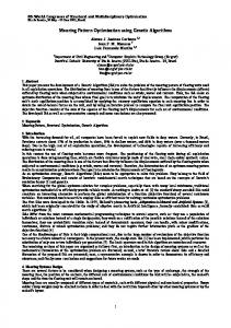
(b) Figure 1. AUC average values with error bars over 20 experiments. (a) Varying p,m while keeping pc constant. (b). Varying pc while keeping p,m constant

629 Table 2. Classification performance of experiments. Rightmost columns show AUC estimate values averaged with standard deviation over a number of experiments. (N: number of experiments, G: number of generations, P: population size, Pc: crossover rate, pm.: mutation rate, pl,,: logarithmic mutation factor)

P

p,

P

P,m

200

0.8

0.2

20

HAT (best in Figlb.)

20

25

200

0.8

0.2

1.0

99.81±1.78

98.26±1.65

Iris

30

30

30

0.8

0.2

0.3

96.04±1.67

89.23±6.82

Iris-noise

30

30

30

0.8

0.2

0.3

91.92±2.77

87.25±6.81

Heart

20

30

30

0.8

0.2

0.3

86.14±1.75

81.32±6.65

Heart-noise

20

30

30

0.8

0.2

0.3

85.36±1.51

77.47±7.28

Random2l

10

30

30

0.8

0.2

0.3

87.80±0.99

86.68±3.07

Repeat2l

10

30

30

0.8

0.2

0.3

89.65±0.99

90.01±3.20

Redund2l

10

30

30

0.8

0.2

0.3

88.49±1.04

86.77±1.81

irs

heart

1

0.95

I

r

I

0.95

F

0.85

0,85

086

0~8

C,

Held-out test 98.26±1.65

HAT(best in Figla.)

-I

0.9

1.0

Cross-validation 99.81±1.78

G 25

N

Dataset

0s

i Ta

0,7

07

0'65

065 0-65

0~75

0.6 II

2

0.55

Best Population

055 4

6

12

10 8 Generations

14

n r, I U..

-1

16

0

0I

4

6

2

4

6

1 A 10

8t 8

Generations

--Best Population I I 12 16 14

(b)

(a)

hat

repeat2l

I

I I

I

095 0,9

-T

r T S

b~~~~~~~~

S:I '-T :

a-ae

11

.: T T.. T 7 1 a1

0. 86

08

0

zi 075 0.7

06.5

0..6 .. ---Best ----- Population

0 55 tiu...;

a 5n10 Generations

_

I

15

__.

20

Generations

(d) (c ) Figure 2. Classification performance over evolutionary time. Plots of average fitness for the best individual

and the mean population are shown for some of the experiments in Table 2. Values are averaged over the number of repetitions, N. (a) Iris dataset, (b) Heart, (c) Repeat2l, (d) HAT.

629

630

In order to study the role of the plm parameter in the quality of solutions found by the logarithmic mutation we carried out further experiments in the HAT dataset. We are particularly interested in studying this experiment because proteomics is a hot topic currently for experimentation in bioinformatics. Besides, this dataset comprises a higher dimensionality than those previously described. We varied Plrn stepwise within a range of 0.2 to 1.0 (Figure la). Note that best classification results over 95% were obtained while setting p, = 0.8 with Plrn = 1.0 . The effect of this value in the mutation factor is that the complete genome, that is, the whole set of scaling factors, is translated in the same direction to a bigger o lower scale, allowing the GA to explore different order of magnitudes during the computation of the weighting parameters. Useful combinations of subsets of weights in dissimilar scales are then propelled by the crossover rate. Hence we studied the effect of changing the crossover rate using the best mutation factor rate of 1.0 (Figure lb). There were not major changes in the classification performance when pc varies from 0.5 to 0.9. Lastly we assesed the practicality of the GA for tuning the kernel parameters by tracing the SVM generalization performance during the evolutionary process. Figure 2 shows plots of AUC vs generations for experiments with the Iris (Fig. 2a), Heart (2b), Repeat2l (2c) and HAT (2d) datasets, averaged over the number of experiments reported in Table 2 (until the maximum number of generations before the algorithm became stalled over the set of experiments). It can be seen a tendency for the AUC to increase as the number of generations grow in all the cases. In the Heart and Repeat21 datasets the trend has a small slope as these are noisy datasets. On the other hand, for the Iris and HAT datasets, there is a sudden increment of both population mean and best chromosome fitness during the initial generations and then it keeps growing gradually showing that the set of parameters searched by the GA improve having a meaningful effect over time. A similar behaviour was observed in the remainder datasets.

5 Conclusions We have described a GA approach for adjusting multiple parameters in SVM kernels. Although we considered weighted RBF kernels, the method can be extended to other weighted kernels. The experiments showed encouraging results in generalization performance for tuning kernels including a few (4, 6) or a large (20, In the latter case 207) number of parameters. parameterization is prohibited in the standard grid-search technique due to computational costs. In the particular case of the HAT proteomic dataset, performance achieved is similar to that reported by our collaborators in a

630

previous study using other machine learning methods not related with weighted kernels or SVM [ 16]. This study showed the applicability of GA for adapting SVM kernels to a particular dataset. However there are interesting questions arising from this approach. For example, we attained a high variability in the results of the held-out tests. When examining the weights given by the best chromosomes evolved for a specific dataset we found that they are very heterogeneous in the scale of magnitude due to the logarithmic mutation that was used. This prompted us to design a different mutation strategy, where the weights are all maintained in a homogenous scale by controlling a single global width parameterized beforehand using a grid-search. Preliminary results of this combined strategy are being reported in an ongoing paper. Other ideas emerging form this work might provide useful insight in outlining new algorithms for tasks like feature subset selection and feature extraction. If the weights encoded in the chromosome represent scale factors of the input variables they can indicate the degree of the relevance of those variables while learning the concept implicit in the dataset. Once the GA has evolved those variables with highest scale factors can be regarded as the most important for solving the given task. We are currently working on this direction by having the GA method described above to apply a cut off threshold on the vector si forcing the less relevant features to zero thus giving sparse weights for the selected features (alternatively they can be ranked by magnitude). Since the kernel weights must be plugged into the SVM during training, this can be considered a wrapper method for feature selection [19] in contrast to other GA approaches where the chromosome encodes the inclusion, or the identification of the variables to be included in a filter method [15, 20]. We intend to use this approach for biomarker discovery (results will be published

elsewhere).

Acknowledgments We would like to thank our team of collaborators Prof. Sanjeev Krishna, Dr. Dan Agranoff and Dr. Marios Papadopoulos at the Department of Cellular and Molecular Medicine, St George's Hospital Medical School, London, UK for allowing us to use the HAT dataset in this preliminary work. Datasets and comprehensive analytical studies will be published elsewhere. We also thank Dr. Mark Herbster, Prof. Anthony Finkelstein (Dept. of Computer Science, UCL, London, UK) and Dr. Anthony A. Holder (Division of Parasitology, National Institute for Medical Research, London, UK) for valuable discussions and providing support for this work. Finally, we are grateful to the reviewers for their usefiul comments.

631

References [1] V. Vapnik, Statistical Learning Theory: John Wiley & Sons, 1998. [2] B. Boser, I. Guyon, and V. Vapnik, "A training algorithm for optimal margin classifiers," presented at 5th Annual ACM Workshop on COLT, 1992. [3] B. Scholkopf, A. Smola, R. C. Williamson, and P. L. Bartlett, "New support vector algorithms," Neural Computation, vol. 12, pp. 1207-1245, 2000. [4] A. Ben-Hur, D. Horn, H. Siegelmann, and V. Vapnik, "Support vector clustering," The Journal of Machine Learning Research, vol. 2, pp. 125-137, 2002. [5] T. Joachims, "Transductive Inference for Text Classification using Support Vector Machines.," presented at Intemational Conference on Machine Learning (ICML), 1999. [6] I. Guyon, J. Weston, S. Barnhill, and V. Vapnik, "Gene Selection for Cancer Classification using Support Vector Machines," Machine Leaming, vol. 46, pp. 389-422, 2002. [7] C. Cortes and V. Vapnik, "Support vector networks," Machine Learning, vol. 20, pp. 273-297, 1995. [8] C. Hsu, C. Chang, and C. Lin, "A Practical Guide to Support Vector Classification," Department of Computer Science and Information Engineering, National Taiwan University 2003. [9] D. Goldberg, Genetic Algorithms in Search, Optimization and Machine Learning.: Addison Wesley, 1998. [10] N. Cristianini and J. Shawe-Taylor, An Introduction to Support Vector Machines and other kernel-based learning methods: Cambridge University Press, 2000. [11] 0. Chapelle, V. Vapnik, 0. Bousquet, and S. Mukherjee, "Choosing Multiple Parameters for Support Vector Machines," Machine Learning, vol. 46, pp. 131-159, 2002. [12] F. Friedrichs and C. Igel, "Evolutionary Tuning of Multiple SVM Parameters," presented at 12th European Symposium on Artificial Neural Networks (ESANN 2004), 2004. [13] T. Fawcett, "ROC Graphs: Notes and Practical Considerations for Researchers," HP Labs Tech Report HPL-2003-4, 2003. [14] C. L. Blake and C. J. Merz, "UCI Repository of machine learning databases," University of California, Department of Computer Science, 1998. [15] E. Cantu-Paz, "Feature Subset Selection, Class Separability and Genetic Algorithms," presented at Genetic and Evolutionary Computation Conference (GECCO-2004), 2004. [16] M. C. Papadopoulos, P. M. Abel, D. Agranoff, A. Stich, E. Tarelli, B. A. Bell, T. Planche, A. Loosemore, S. Saadoun, P. Wilkins, and S. Krishna, "A novel and accurate test for Human African Trypanosomiasis," Lancet, vol. 363, pp. 1358-1363, 2004. [17] J. Weston, A. Elisseeff, G. BakIr, and F. Sinz, "SPIDER: object-orientated machine learning library,

version 1.51," Department of Empirical Inference for Machine Learning and Perception, Max Planck Institute for Biological Cybernetics, 2004. [18] T. Joachims, "Making large-scale SVM learning practical," in Advances in Kernel Methods - Support Vector Learning, B. Sholkopf, C. Burges, and A. Smola, Eds.: MIT Press, 1999. [19] I. Guyon and A. Elisseeff, "An introduction to variable and feature selection.," Journal of Machine Learning Research, vol. 3, pp. 1157-1182, 2003. [20] H. Frohlich, 0. Chapelle, and B. Scholkopf, "Feature Selection for Support Vector Machines by Means of Genetic Algorithms," presented at IEEE 15th International Conference on Tools with Artificial Intelligence (ICTA 2003), 2003.

631