Evolution of perturbations and cosmological constraints in ... - CiteSeerX

arXiv:1402.2972v1 [astro-ph.CO] 12 Feb 2014

Prepared for submission to JCAP

Evolution of perturbations and cosmological constraints in decaying dark matter models with arbitrary decay mass products Shohei Aoyama,1 Toyokazu Sekiguchi,1,2 Kiyotomo Ichiki3 and Naoshi Sugiyama1,3,4 1

Department of Physics and Astrophysics, Nagoya University, Nagoya 464-8602, Japan University of Helsinki and Helsinki Institute of Physics, P.O. Box 64, FI-00014, Helsinki, Finland 3 Kobayashi-Maskawa Institute for the Origin of Particles and the Universe, Nagoya University, Nagoya 464-8602, Japan 4 Kavli Institute for the Physics and Mathematics of the Universe (Kavli IPMU), The University of Tokyo, Chiba 277-8582, Japan 2

Abstract. Decaying dark matter (DDM) is a candidate which can solve the discrepancies between predictions of the concordance ΛCDM model and observations at small scales such as the number counts of companion galaxies of the Milky Way and the density profile at the center of galaxies. Previous studies are limited to the cases where the decay particles are massless and/or have almost degenerate masses with that of mother particles. Here we expand the DDM models so that one can consider the DDM with arbitrary lifetime and the decay products with arbitrary masses. We calculate the time evolutions of perturbed phase-space distribution functions of decay products for the first time and study effects of DDM on the temperature anisotropy in the cosmic microwave background and the matter power spectrum at present. From a recent observational estimate of σ8 , we derive constraints on the lifetime of DDM and the mass ratio between the decay products and DDM. We also discuss implications of the DDM model for the discrepancy in the measurements of σ8 recently claimed by the Planck satellite collaboration.

Keywords: dark matter, cosmological perturbation theory, large scale structure

Contents 1 Introduction

1

2 Model of DDM and Boltzmann equation 2.1 DDM model and set up 2.2 Boltzmann equations 2.2.1 Mother particles 2.2.2 Daughter particles

3 3 4 6 7

3 Time evolutions of perturbations 3.1 A case of non-relativistic decay 3.1.1 Perturbations crossing the 3.1.2 Perturbations crossing the 3.2 A case of relativistic decay 3.2.1 Perturbations crossing the 3.2.2 Perturbations crossing the

horizon after the decay time horizon before the decay time horizon after the decay time horizon before the decay time

9 9 9 11 13 13 14

4 Signatures in cosmological observables 4.1 Effects on Cl 4.2 Effects on P (k)

15 15 19

5 Discussion 5.1 Implication on the anomaly in estimated σ8 from Planck

20 24

6 Conclusion

25

A Initial condition for the perturbed distribution functions of the daughter particles 26 A.1 Radiation-dominated era 27 A.2 Matter-dominated era 28

1

Introduction

Numerous kinds of astrophysical observations suggest the existence of dark matter, which has no electro-magnetic or strong interactions with other particles in the Universe. It is necessary for explaining the observed phenomena such as flat rotation curves of galaxies, anisotropies in the cosmic microwave background (CMB) and the formation of large scale structure within the age of the Universe, tage = 13.8 Gyr [1]. In particular, to explain the hierarchical formation of the cosmic structure, dark matter should have very small momentum hence so-called cold dark matter (CDM) becomes the standard model of dark matter. However, while it is widely believed that dark matter consists of particles beyond the Standard Model, we have little knowledge on the nature of dark matter. Thus, for

–1–

example, it remains possible that dark matter decays into other particles with smaller masses. This kind of dark matter is called decaying dark matter (DDM). By constraining the lifetime of DDM, we can obtain the nature of dark matter and information about a particle theory lying behind it. While the CDM model is widely consistent with observations on cosmological scales, there exist some discrepancies at sub-galactic scales between the model predictions by N-body simulations and astronomical observations. Well known examples are the ”cusp problem” [2], i.e., the over-concentration problem of the inner core of galaxies, and the ”missing satellite problem” [3] or the ”too big to fail problem” [4], where the number or properties of satellite galaxies of the Milky Way do not match the results from numerical simulations. DDM is often discussed as a remedy to such small-scale CDM problems, for example, see Cen [5]. The DDM model, however, should pass the tests from precise cosmological observations, such as measurements of the CMB and the large scale structure of the universe. One of the aims of this paper is therefore to give a complete set of perturbation equations of the DDM model with decay products having arbitrary masses, and show some evolutions of density perturbations in the DDM model to compare them with recent cosmological observations. Cosmological implications of DDM have been studied by several authors [5–20]. Among them, Kaplinghat [9] and Huo [18] have considered models in which dark matter decays into two ”daughter” particles1 well before the matter-radiation equality epoch. They calculated time evolution of perturbations and set constraints on the mass ratio and the life time of DDM from the free streaming scale of daughter particles. The former considered the DDM which decays into a massive particle and massless one in the early Universe. They computed the matter power spectrum and discussed the effects of free-streaming of the decay products by considering the phase-space density of the massive daughter particle. The latter computed the CMB power spectrum in addition to the matter power spectrum. Moreover, DDM models in which the mass difference between the mother and the massive daughter particles ∆m is much smaller than the mass of the mother particles are studied in refs. [16, 17, 20, 21]. In particular, Peter [16] has considered effects of the recoil energy of the daughter particles on the halo mass-concentration and galaxy-cluster mass function using N-body simulations and set constraints on the lifetime of DDM and ∆m in terms of the kick velocity vkick by demanding that the daughter particles in halos with mass M = 1012 M⊙ do not escape from the halos and destroy the gravitational potential. She also set constraints by using weak lensing measurements and X-ray observations. Wang et al. have analyzed Nbody simulations with DDM and focused on the statistical properties of the transmitted Lyman-α (Ly-α) forest flux. By comparing the data of the Sloan Digital Sky Survey (SDSS) and WMAP 7 with their simulation data, they set a constraint on the life time of DDM as Γ−1 > 40 Gyr where vkick & 50 km/s [21]. However, previous studies so far could not deal with DDM models where mother particles decay into particles with arbitrary mass at late times (i.e. after the matter-radiation equality). This is what we will explore in this paper. In this paper, we investigate models of DDM which decays into two daughter 1

We call progenitor particle ”mother” particle.

–2–

particles. We study linear cosmological perturbations in the DDM model without approximations such that the decay products are massless or highly non-relativistic. Instead, we directly solve the Boltzmann equations for the mother and daughter particles and follow the time evolutions of their distribution functions in the discretized phase space. In this formulation, one can set masses of both daughter particles to arbitrary values. While our formulation and numerical implementation can deal with arbitrary lifetime and/or masses of daughter particles, to minimize complication, we assume that DDM decays after cosmological recombination into two particles one of which has a finite mass and the other is massless. Here, we basically follow the notation of Ma and Bertschinger [22]. We adopt natural units with c = ~ = kB = 1. The proper and conformal time are denoted by t and τ , respectively. A dot represents partial derivative with respect to the conformal time, i.e., f˙ ≡ ∂f /∂τ . A quantity with a subscript ”∗” indicates its value at cosmological recombination. The layout of this paper is as follows. In the following section, we introduce our DDM model and present the Boltzmann equations, which describe the perturbation evolutions. In addition, we also describe how we solve the equations numerically. Section 3 denotes time evolutions of perturbations in the DDM model. Effects on cosmological observables including the angular power spectrum of the CMB anisotropy Cl and the matter power spectrum P (k) are discussed in section 4. In section 5, we discuss some interpretations for the effects of the decay of dark matter and derive a constraint on the DDM model from an observed value of σ8 . Finally, section 6 concludes this paper.

2 2.1

Model of DDM and Boltzmann equation DDM model and set up

In this work, we consider a model of DDM (M) which decays into two particles (D1, D2) well after cosmological recombination, M → D1 + D2 (with Γ−1 ≫ t∗ ) ,

(2.1)

where Γ is the decay rate of DDM. Throughout this paper, we assume a variant of the concordance flat power-law ΛCDM model where CDM is replaced with DDM, and consider cosmological perturbations. The model is specified with the following cosmological parameters: (Ωb , ΩM∅ , h∅ , τreion , ns , As , Γ, mD1 /mM , mD2 /mM ),

(2.2)

where Ωb and ΩM∅ are the density parameters of baryons and mother particles, respectively, h∅ is the reduced Hubble constant estimated assuming that the DDM does not decay, τreion is the optical depth of reionization, and ns and As are respectively the spectral index and amplitude of the primordial curvature perturbation at k = 0.002 Mpc−1 . Here and in the following, the subscript ∅ indicates quantities

–3–

which are estimated assuming Γ = 0. Following the WMAP 7-year results [23]2 , we fix (Ωb , ΩM∅ , h∅ , τreion , ns , As ) to (0.0454, 0.226, 0.704, 0.088, 0.967, 2.43 × 10−9 ). With the parameterization eq. (2.2), the genuine Hubble constant h and the density parameter of mother particles ΩM are derived parameters which can be obtained by solving the background evolution. It should be noted that these values of parameters are not necessary to be the best fitting values to WMAP-7 year data in the DDM model. These values are adopted only for a reference. Regarding mD2 /mM , while the formalism we present in this section is applicable for arbitrary masses of the daughter particles, as is stated in introduction, we in the rest of this paper assume that the mass of one of the daughter particles can be nonzero and the other one is massless. Thus, Γ and mD1 /mM are treated as free parameters with mD2 /mM being fixed to zero. Subscripts ”M”, ”D1” and ”D2” indicate the mother, massive daughter, and massless daughter particles, respectively. 2.2

Boltzmann equations

In this paper, we choose the synchronous gauge of the mother particles to describe cosmological linear perturbations. The line element is given by  ds2 = a(τ )2 dτ 2 + (δij + hij (x, τ )) dxi dxj , (2.3)

where a is the scale factor and hij represents the metric perturbations. In terms of Fourier components, hij can be given as   Z 1 3 ˆik ˆ j + 6ηT (k, τ )(k ˆ ik ˆ j − δij ) exp(ik · x) , hij (x, τ ) = d k hL (k, τ )k (2.4) 3

ˆ is a wave number vector and k ˆ is the unit vector of k. In the rest of where k ≡ k k this section, we focus on a single mode of perturbations with k and often abbreviate dependences of perturbed variables on k. The Boltzmann equation which describes time evolution of a phase-space distribution function f (x, q, τ ) can be written as   dxi ∂f dq ∂f dni ∂f ∂f ∂f , (2.5) + + + = i i ∂τ dτ ∂x dτ ∂q dτ ∂n ∂τ C where q is the comoving momentum, which is related to the physical momentum p by q = ap, and q and ni = q i /q are respectively the norm and the direction of q. For a perturbation mode with k, the second term of the left hand side can be rewritten ˆ · n) (q/ε) f , where ε is the comoving energy. In the left hand side, the third as i(k term can be rewritten in terms of the metric perturbations by adopting the geodesic equation dpµ p0 + Γµ αβ pα pβ = 0 . (2.6) dτ 2

Recently, the cosmological parameters derived by Planck have been reported [24]. Since the estimated values of Ωb h2 and Ωc h2 change from those of the WMAP 7-year results only by several percent, results and constraints presented in this paper may not be affected significantly when the cosmological parameters from Planck are adopted.

–4–

In particular, time-component (µ = 0) of eq. (2.6) gives dq/dτ as  dq 1 ˙ ˆ · n)2 . hL + 6η˙ T (k = η˙ T − dτ 2

(2.7)

fM (q, n, τ ) = NM (τ )δ (3) (q) ,

(2.8)

The fourth term of the left hand side of eq. (2.5) can be neglected to the first order, because both (dni /dτ ) and (∂f /∂ni ) are first-order quantities in the flat Universe. The right hand side of eq. (2.5) is the collision term, which also describes effects of decay or creation of particles on the distribution function. Aoyama et al. [25] provided those for the mother and daughter particles. In this paper, we assume that momenta of the mother particles are negligibly small compared with the mass. Under this assumption in conjunction with our choice of gauge, the distribution function of the mother particles should be proportional to the delta function of q. Then we obtain

where NM is the comoving number density of the mother particles. Then the collision terms can be recast into [25]   ∂fM M: = −aΓfM , (2.9) ∂τ C   aΓNM ∂fDm = δ (q − apDmax ) , (2.10) Dm : ∂τ 4πq 2 C where pDmax is the initial physical momentum of decay particles in the rest flame of the mother particles, which is given by pDmax

" #1/2
(m2D1 + m2D2 )2 1 2 2 2 = mM − 2 mD1 + mD2 + . 2 m2M

(2.11)

Note that collision terms are the same for both the daughter particles. For later convenience, we introduce τq which is the conformal time when the daughter particles with a comoving momentum q are produced, i.e., q = a(τq )pDmax .

(2.12)

From eqs. (2.7), (2.9) and (2.10), the Boltzmann equations for the mother and the daughter particles can be written as    ∂fM 1 ˙ qk ˆ ∂fM 2 ˆ M: η˙ T − , hL + 6η˙ T (k · n) = −aΓfM (2.13) + i (k · n)fM + q ∂τ εM ∂q 2    ∂fDm 1 ˙ qk ˆ ∂fDm 2 ˆ Dm : η˙ T − (2.14) hL + 6η˙ T (k · n) +i (k · n)fDm + q ∂τ εDm ∂q 2 aΓNM δ (apDmax − q) , = 4πq 2

–5–

where εM (εDm ) is the comoving energy of the mother (m-th daughter) particles. We divide a distribution function f into the background f and the perturbation ∆f as fM (q, k, n, τ ) = f M (q, τ )δ (3) (k) + ∆fM (q, k, n, τ ) , fDm (q, k, n, τ ) = f Dm (q, τ )δ (3) (k) + ∆fDm (q, k, n, τ ) ,

(2.15) (2.16)

where f depends only on q and τ . Due to the isotropy of the background geometry, ∆f ˆ · n) with l ≥ 0. Therefore can be expanded in terms of the Legendre polynomials Pl (k we can define ∆fM(l) (∆fDm(l) ) as the l-th multipole moment of ∆fM (∆fDm ), i.e. ∆fM (q, n, τ ) = ∆fDm (q, n, τ ) =

+∞ X

l=0 +∞ X l=0

2.2.1

ˆ · n), (−i)l (2l + 1)∆fM(l) (q, τ )Pl (k

(2.17)

ˆ · n) . (−i)l (2l + 1)∆fDm(l) (q, τ )Pl (k

(2.18)

Mother particles

By substituting eq. (2.15) into eq. (2.5), we obtain the Boltzmann equations for the mother particles as follows: unperturbed : f˙ M = −aΓf M , (2.19)     ∂∆fM ∂f M 1 ˙ qk ˆ 2 ˆ 1st order : η˙ T − + i (k · n)∆fM + q hL + 6η˙ T (k · n) ∂τ εM ∂q 2 = −aΓ∆fM . (2.20) From eqs. (2.8) and (2.19), we obtain f M (q, t) =

N M (τ ) δ(q) 4πq 2

(2.21)

where N M (τ ) ∝ exp (−Γt) is the mean comoving number density of the mother particles. Denoting the mean comoving number density of the mother particles without decay as N M∅ , N M can be given as N M (τ ) = N M∅ exp (−Γt) .

(2.22)

Note that N M∅ is constant. According to our gauge choice, the dipole moment of the mother particles is zero. Since the mother particles do not have nonzero momentum distribution, higher-order multipole moments should vanish, i.e., ∆fM(l) = 0 (for l ≥ 1) .

(2.23)

On the other hand, from eqs. (2.17) and (2.20), the monopole moment ∆fM(0) obeys the following equation, ∂∆fM(0) ∂f 1 = h˙ L q M − aΓ∆fM(0) . ∂τ 6 ∂q

–6–

(2.24)

Equations (2.19) and (2.24) can be recast into evolution equations for the mean energy density ρ¯M and its perturbation ρ¯M δM , which are defined as Z 1 ρM ≡ 4 dq 4πq 2εM f M , (2.25) a Z 1 ρM δM ≡ 4 dq 4πq 2εM ∆fM(0) . (2.26) a Then by integrating eqs. (2.19) and (2.24) multiplied by 4πq 2 εM /a4 , we obtain d ρ¯M + 3H¯ ρM = −aΓ¯ ρM , dτ h˙ L d [¯ ρM δM ] + 3H¯ ρM δM = − ρ¯M − aΓ¯ ρM δM , dτ 2

(2.27) (2.28)

where H = a/a ˙ is the conformal Hubble expansion rate. In combination, these two equations lead to h˙ L δ˙M = − . (2.29) 2 We note that eq. (2.29) is the same as that for CDM without decay [22]. We also note that ρ¯M as ρ¯M (τ ) = mM N M (τ )/a3 since the mother particles are non-relativistic. 2.2.2

Daughter particles

By substituting eq. (2.16) into eq. (2.14), one can find ∂f Dm aΓN M = δ(τ − τq ) , (2.30) ∂τ 4πq 3 H    ∂∆fDm 1 ˙ qk ˆ ∂f Dm 2 ˆ 1st order : η˙ T − hL + 6η˙ T (k · n) +i (k · n)∆fDm + q ∂τ εDm ∂q 2 aΓN M δM δ(τ − τq ) . (2.31) = 4πq 3 H

unperturbed :

In deriving these equations, we used a relation δ(q − apDmax ) =

1 δ(τ − τq ). qH

(2.32)

As seen from eq. (2.30) and (2.31), the unperturbed and first order perturbation equations for both the daughter particles are identical [9, 20, 25]. Therefore we can write f D1 (q, τ ) = f D2 (q, τ ) ≡ f D (q, τ ) .

(2.33)

As in previous works [20, 25], by solving eq. (2.30), we obtain f D (q, τ ) =

aq ΓN M (τq ) Θ (τ − τq ) , 4πq 3 Hq

–7–

(2.34)

where aq = a(τq ), Hq = H(τq ) and Θ(x) is the Heaviside function. Equation (2.31) can be expanded in terms of multipole moments, which leads to a Boltzmann hierarchy for the daughter particles: ∂ (∆fDm(0) ) ∂τ ∂ (∆fDm(1) ) ∂τ ∂ (∆fDm(2) ) ∂τ ∂ (∆fDm(l) ) ∂τ

∂f qk 1 aΓN M ∆fDm(1) + h˙ L q D + δM δ (τ − τq ) , εDm 6 ∂q 4πq 3 H
qk ∆fDm(0) − 2∆fDm(2) , = 3εDm  
qk 2 ∂f 1 ˙ 2∆fDm(1) − 3∆fDm(3) − = hL + η˙ T q D , 5εDm 15 5 ∂q
qk l∆fDm(l−1) − (l + 1)∆fDm(l+1) = (for l ≥ 3) (2l + 1)εDm =−

(2.35) (2.36) (2.37) (. 2.38)

By using ∆fDm(0) , ∆fDm(1) , ∆fDm(2) , the perturbed energy density δρ = ρδ, perturbed pressure δp = pπL , energy flux θ and shear stress σ can be written as Z 1 (2.39) ρDm δDm ≡ 4 dq 4πq 2 εDm ∆fDm(0) , a Z q2 1 ∆fDm(0) , (2.40) pDm πLDm = 4 dq 4πq 2 3a εDm Z k (ρDm + pDm ) θDm = 4 dq 4πq 2 q∆fDm(1) , (2.41) a Z 2 1 2 q (ρDm + pDm ) σDm = 4 dq 4πq ∆fDm(2) , (2.42) a εDm where ρDm and pDm are the mean energy density and pressure of the m-th daughter particles, respectively. Here, πLDm , θLDm and σDm are higher-order velocity-weighted quantities since phase space integral in these are weighted by the velocity q/ε or velocity squired (q/ε)2 compared with the density perturbation δDm . Equations (2.35)-(2.38) are the same as those for massive neutrinos except for the last term in eq. (2.35) (see ref. [22]), which is responsible for the creation of density perturbation of the daughter particles from that of the mother ones. While the structure of the perturbation equations may not seem to differ from that of massive neutrinos significantly, in fact their solution is far more complicated. The complication arises from the source terms (the second and third terms in the right hand side of in eq. (2.35) and the last term in eq. (2.37)). These terms contain delta functions on τ , which clearly require a specialized treatment in numerical computation. In order to solve the perturbation equations and obtain the CMB angular power spectrum Cl as well as the matter power spectrum P (k) we modified the publicly available CAMB code [26]. In order to calculate the time evolutions of the perturbed distribution functions of the daughter particles ∆fDm(l) , the comoving momentum q is discretized into 1024 nodes for each daughter particle. The q-nodes are distributed uniformly in the logarithmic scale for 10−7 pDmax ≤ q ≤ 0.03 pDmax and in the linear scale for 0.03 pDmax ≤ q ≤ pDmax . The maximum multipole is set to be 45.

–8–

The initial conditions of ∆fDm(l) (q, τ ) are set as follows. When τ < τq , both daughter particles which have comoving momentum q have never been generated. Thus f D (q, τ ) = ∆fD (q, n, τ ) = 0 (for τ < τq ).

(2.43)

and (2.37), thesource terms (1/6)h˙ L q(∂f D /∂q), (aΓN M /4πq 3H)δM δ(τ − In eqs. (2.35)  τq ) and (1/15)h˙ L + (2/5)η˙ T q∂f D /∂q contain a delta function δ(τ −τq ), which makes ∆fDm(0) and ∆fDm(2) arise like a step function at τ = τq . In order to treat these terms, we obtain the initial values by integrating eqs. (2.35) and (2.37) with τ in a infinitesimal interval around τ = τq . The initial values of ∆fDm(0) and ∆fDm(2) are provided in eqs. (A.5) and (A.7) in Appendix A. For τ > τq , q∂ f¯D /∂q becomes a smooth function of τ and the time evolutions of the perturbed distribution functions of the daughter particles can be calculated in the same way as massive neutrinos in the standard cosmology.

3

Time evolutions of perturbations

In this section, we discuss time evolutions of perturbed quantities. Hereafter we continuously assume that mD2 is zero, while the mass of the first daughter particles mD1 can vary in [0, mM ]. For later convenience, we respectively denote the scale factor at the decay time and the horizon crossing as ad and ahc , i.e., t(ad ) ≡ Γ−1 and τ (ahc ) ≡ πk −1 . 3.1

A case of non-relativistic decay

In this subsection, we consider a case with mD1 ≃ mM , which we refer to as nonrelativistic decay. As a representative value, we here adopt mD1 = 0.999 mM , with which the massive daughter particles are produced with a velocity kick vkick ≃ 1 − mD1 /mM = 0.001. We expect time evolutions of perturbations depend on whether the scale of perturbations is inside or outside the horizon, as well as whether the DDM has decayed or not. Therefore in what follows we separately investigate cases with ad < ahc and ad > ahc . 3.1.1

Perturbations crossing the horizon after the decay time

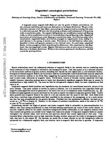
Let us first consider perturbations which cross the horizon after the decay of DDM, i.e. ad < ahc . Here we adopt Γ−1 = 6 Myr and consider evolutions of perturbations at k = 8 × 10−4 hMpc−1 . This setup corresponds to ad ≃ 5 × 10−3 and ahc ≃ 0.1. In figure 1, we plot time evolutions of perturbation quantities of the mother and daughter particles, including density perturbations δi , pressure ones πLi , energy fluxes θi and shear stresses σi . Note that regarding perturbed quantities of the mother particles, only the density perturbation δM is nonzero due to the vanishing momentum distribution of the mother particles and our choice of gauge. Before the decay of DDM a < ad , the density perturbations of the daughter particles δD1 and δD2 grow in proportion to δM . It is because monopole moments ∆fDm(0) are sourced by the density perturbation of the mother particles δM and the metric perturbation hL , which also grow during the matter-domination epoch. In

–9–

t~Γ-1 ad 5×10-3

10-3

10-2

10-1

10-3

10-2

10-1

102 100 10-2 10-4 10-6 10-8 10-10 100 10-2 10-4 10-6 10-8 10-10

(1+wi)σi [h-3Mpc3]

wiπLi [h-3Mpc3]

δi [h-3Mpc3]

horizon crossing ahc 1×10-1

(1+wi)θi [h-2Mpc2]

102 100 10-2 10-4 10-6 10-8 10-10 100 10-2 10-4 10-6 10-8 10-10

t~Γ-1 ad 5×10-3

horizon crossing ahc 1×10-1

100

Figure 1. Time evolutions of perturbations in the case of non-relativistic decay. Here we show perturbations whose scale k = 8 × 10−4 hMpc−1 crosses the horizon after the decay time Γ−1 = 6 Myr. Shown are the density perturbations (top left), energy fluxes (top right), pressure perturbations (bottom left) and anisotropic stresses (bottom right) of the mother (blue solid line), massive daughter (red dashed line) and massless daughter (green dot-dashed line) particles. In the upper left panel, the line of the density perturbation of the massive daughter overlaps that of the mother particle. Two dotted vertical lines indicate the horizon crossing and the decay time. wi = pi /ρi is the equation of state of the i-th component. According to our gauge choice, the dipole and quadrupole moment of the mother particle are zero. Thus the energy flux and anisotropic stress of mother particle are zero. In addition, because of our assumption that the momentum of mother particle is negligible compared with its mass, the pressure perturbation of mother particle becomes zero. Therefore these quantities of mother particle, such as θM , πM and σM , are zero and not shown in upper right and bottom panels.

particular, sufficiently prior to the decay time in the matter-dominated Universe, δD1 and δD2 are related to δM as δD1 = δM , (3.1) 23 δM , (3.2) δD2 = 21 on superhorizon scales, which can be derived analytically as in Appendix A. Our numerical result is consistent with analytic one as seen in the upper left panel of figure 1.

– 10 –

Since the massive daughter particles are non-relativistic, their pressure perturba2 tions are suppressed as δpD1 ≃ O(vkick )δρD1 , while that of the massless daughter one is large as δpD2 = δρD2 /3. As can be seen in eq. (2.36) dipole moments ∆fDm(1) are sourced only by monopole and quadrupole moments via free-streaming. At superhorizon scales k < πτ −1 , therefore dipole moments ∆fDm(1) and hence the energy fluxes θDm are little generated. On the other hand, as quadrupole moments ∆fDm(2) are directly generated by metric perturbations (see eq. (2.36)), σDm can be large. In addition, for the same reason as the pressure perturbation δpD1 , velocity-weighted quantities of the massive daughter particles, including θD1 and σD1 , are further suppressed. After the decay of DDM but still before the horizon crossing ad < a < ahc , daughter particles are no longer sourced by the mother particles and the last term of eq. (2.35) becomes negligible. In this epoch, the Boltzmann equations for the daughter particles become the same as that for collisionless free-streaming particles, e.g. massive neutrinos (see ref. [22]). For non-relativistic particles, the evolution equation of ∆fD1 should be effectively reduced to that of CDM. Hence the density fluctuation of the massive daughter particles evolves in the same way as the mother ones. Due to redshifting of physical momenta, higher-order velocity-weighted quantities such as πLD1 , θD1 and σD1 decrease afterward. For the massless daughter particles, the evolution equation of ∆fD2 becomes the same as that of massless neutrinos. After the horizon crossing a > ahc , the daughter particles start free-streaming. The free-streaming length of the massless daughter particles equals to the size of horizon and perturbation quantities decay oscillating. For massive daughter particles, the density perturbation δD1 continues to grow inside the horizon in the same way as CDM, while the velocity-weighted quantities continue to decay due to redshifting of momentum. 3.1.2

Perturbations crossing the horizon before the decay time

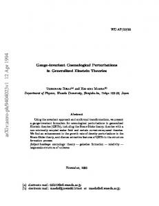
Now we move to a case where DDM decays inside the horizon. We set the decay time to Γ−1 = 0.1 Gyr, which corresponds to ad ≃ 3 × 10−2 , and investigate perturbations on a scale k = 8 × 10−3 hMpc−1 , which crosses the horizon at ahc ≃ 2 × 10−3. Time evolutions of perturbed quantities related to the mother and daughter particles are plotted in figure 2. By comparing figure 2 with figure 1, we can say that at superhorizon scales when a < ahc and in this case inevitably before the decay, behaviors of perturbed quantities of the mother and daughter particles are qualitatively the same as in the previous case where the horizon crossing occurs after the decay. In particular, the analytical solutions of eqs. (3.1) and (3.2) again hold at superhorizon scales, which can be qualitatively confirmed in the upper left panel of figure 2. On the other hand, evolutions of perturbations inside the horizon drastically differ from those in the previous case. After the horizon crossing but still before the decay ahc < a < ad , the massless daughter particles start to free-stream. However, as we can see in figure 2, the perturbation quantities, such as δD2 , θD2 and σD2 do not start to oscillate nor decay, contrary to those in figure 1. This is because the monopole moment of the massless daughter particles ∆fD2(0) is continuously sourced by the density per-

– 11 –

δi [h-3Mpc3]

10

102

100

100

10-2

10-2

10-4

10-4

10-6

10-6

100

100

10

-2

10

-2

10-4

10-4

10-6

10-6

10-3

10-2

a

10-1

10-3

10-2

a

10-1

(1+wi)σi [h-3Mpc3]

wiπLi [h-3Mpc3]

horizon crossing t~Γ-1 ahc 2×10-3 ad 3×10-2

(1+wi)θi [h-2Mpc2]

horizon crossing t~Γ-1 ahc 2×10-3 ad 3×10-2 2

100

Figure 2. Same as in figure 1 but for Γ−1 = 0.1 Gyr and k = 8 × 10−3 hMpc−1 . In the upper left panel, the line of the density perturbation of the massive daughter overlaps that of the mother particle as same as figure 1.

turbation of the mother particles, and then the dipole and higher multipole moments are also continuously sourced by ∆fD2(0) . Therefore perturbation quantities of freestreaming relativistic particles keep on growing even inside the horizon. Moreover, as for the massive daughter particles, higher-order velocity-weighted quantities including πLD1 , θLD1 and σLD1 also grow. This is because the massive daughter particles with the nonzero velocity vkick = 0.001 keep on being produced, and these particles with relatively large momenta free-stream to make higher-order velocity-weighted quantities grow continuously in addition to the density perturbation δρD1 . Finally at a > ad , when there are few mother particles to decay, the source terms in the Boltzmann eqs. (2.35)-(2.38) for the daughter particles become ineffective and these particles behave as collisionless free-streaming particles. Perturbation quantities of the massless daughter particles start to oscillate and decay due to free-streaming. Comparing figure 2 with figure 1, we can see perturbation quantities of the massless daughter particles decay more quickly and effects of free-streaming are more prominent than the previous case. This is because most of the daughter particles are produced when a ≃ ad and these particles immediately free-stream over distances larger than the perturbation scale. On the other hand, since the massive particles are non-relativistic, effects of free-streaming is not significant and higher-order velocity-weighted quantities

– 12 –

decrease mostly due to redshifting of momentum. 3.2

A case of relativistic decay

In this subsection, we consider a case with mD1 ≪ mM , which we refer to as relativistic decay. Here we adopt mD1 = 0.1mM , which gives a velocity kick of the massive daughter particles vkick ≃ 1 − 2(mD1 /mM )2 = 0.98. In the same way as section 3.1, we in the following explore time evolutions of perturbations in cases with ad < ahc and ahc < ad separately. 3.2.1

Perturbations crossing the horizon after the decay time

102 101 100 10-1 10-2 10-3 10-4

10-1

10-1

10-2

10-2

10-3 10-3

10

-2

a

10

-1

10

-3

10

-2

a

10

-1

10-3

(1+wi)σi [h-3Mpc3]

wiπLi [h-3Mpc3]

102 101 100 10-1 10-2 10-3 10-4

t~Γ-1 horizon crossing ad 5×10-3 ahc 5×10-2

t~Γ-1 horizon crossing ad 5×10-3 ahc 5×10-2

(1+wi)θi [h-2Mpc2]

δi [h-3Mpc3]

Let us see time evolutions of perturbations whose scale crosses the horizon after the decay time. We adopt a decay time Γ−1 = 6 Myr and the scale of perturbations is fixed to k = 8 × 10−4 hMpc−1 . These parameters lead to ad = 5 × 10−3 and ahc = 5 × 10−2 . Figure 3 shows time evolutions of perturbation quantities of the mother and daughter particles.

0

10

Figure 3. Same as in figure 1 but for mD1 /mM = 0.1.

First of all, we expect cosmological effects of the two daughter particles are identical as long as both of them are sufficiently relativistic. Noting that momenta of particles scale as a−1 , the time when most of the p massive daughter particles become non2 relativistic can be estimated as anr = (vkick / 1 − vkick )ad , which is roughly 2.5 × 10−2 – 13 –

with the parameter values we adopted here. Therefore when a < anr , perturbation quantities of the two daughter particles are almost the same, which can be confirmed in figure 3. One big difference from the case of non-relativistic decay is that the density perturbations δi grow more rapidly after the decay at superhorizon scales as can be seen in the upper left panel of figure 3. The reason can be understood as follows. Since the decay products are relativistic, the Universe is effectively dominated by radiation after the decay. Therefore, as in the radiation-dominated epoch, density perturbations grow as a2 at superhorizon scales instead of a in the matter-dominated epoch (see eqs. (A.9) and (A.20)). As seen in the ΛCDM model with low Ωm (we refer to, e.g., ref. [27]), this leads to an enhancement in the matter power spectrum at scales which crosses the horizon after the matter-radiation equality. This issue will be discussed further in section 4.2. After horizon crossing, even when a > anr , due to the non-vanishing velocity and free streaming of daughter particles, at first growth of δD1 is slower compared with the case of non relativistic decay (see also the upper left panel of figure 1). This leads that the density perturbation of the mother particles δM also grows less, for the gravitational potential sourced by δD1 decays inside the horizon. After the massive daughter particles become fully non-relativistic, their density perturbation starts to grow as CDM does. Other perturbation quantities with higher velocity-weights such as πLD1 , θD1 and σD1 start decreasing almost monotonically without violent oscillations, which is also seen in cases of non-relativistic decay (see the upper right and bottom panel of figure 1). The massless particles keep on free-streaming and their perturbations except for velocity divergence continuously decay. 3.2.2

Perturbations crossing the horizon before the decay time

Figure 4 shows time evolutions of perturbations for a case where the decay occurs inside the horizon. Here we adopt Γ−1 = 0.1 Gyr and show perturbations at a scale k = 8×10−3 hMpc−1 . These parameters correspond to ad ≃ 3×10−2 and ahc = 2×10−3 . In this case, p most of the massive daughter particles become non-relativistic at around 2 anr = (vkick / 1 − vkick )ad ≃ 0.15. At a < anr , as expected, the perturbation evolutions of the two daughter particles are again almost the same, which can be seen in figure 4. As is discussed in the case of non-relativistic decay in section 3.1, in this case perturbation quantities continuously grow inside the horizon until the mother particles completely decay, and then effects of free-streaming become significant. This can be confirmed in figure 4. As the massive daughter particles become non-relativistic at a > anr their density perturbation δD1 starts to grow and other velocity-weighted perturbations πLD1 etc. start to decrease with less oscillation than before. However, the decay of δD1 is so significant, the density perturbation of total matter becomes much smaller than the density perturbations of the mother particles δM . This decay of the density perturbation leads to a significant suppression in the matter power at small scales as will be shown in section 4.2. On the other hand, the massless daughter particles continuously free-stream.

– 14 –

10 102 101 100 10-1 10-2 10-3

103 102 101 100 10-1 10-2 10-3

100

100

10-1

10-1

10-2

10-2

10-3 -3 10

10

-2

a

10

-1

10

-3

10

-2

a

10

-1

-3 10 0 10

(1+wi)σi [h-3Mpc3]

wiπLi [h-3Mpc3]

horizon crossing t~Γ-1 ahc 2×10-3 ad 3×10-2

(1+wi)θi [h-2Mpc2]

δi [h-3Mpc3]

horizon crossing t~Γ-1 -3 -2 3 ahc 2×10 ad 3×10

Figure 4. Same as in figure 2, but for mD1 /mM = 0.1. Some jaggy features on plots are caused by the numerical error on the calculation.

4 4.1

Signatures in cosmological observables Effects on Cl

In this subsection, we consider the CMB power spectrum Cl in the DDM models with Γ−1 > t∗ . In figure 5, we plot the CMB temperature power spectrum ClTT with various decay times 0.01 < Γ−1 [Gyr] < 100 and mass ratios 0.3 < mD1 /mM < 0.9. From the figure, we can see effects of DDM on ClTT are twofold. First one is the shift of the positions of the acoustic peaks caused by a change in the background expansion. The other is the integrated Sachs-Wolfe effect induced by the decay of the gravitational potential. Let us first investigate the effects on positions of the acoustic peaks. When Γ−1 is shorter than the age of the Universe at present tage ≃ 14 Gyr [24] and DDM decays into the relativistic daughter particles, energy density in the Universe and hence the expansion rate stay below those in the ΛCDM model. This makes angular diameter distances larger and hence the angular size of the sound horizon smaller than in the case of the ΛCDM model. Therefore positions of the acoustic peaks shift toward higher l. Second, let us move to the effects that arises at large angular scales larger than

– 15 –

TT

l(l+1)Cl /2π[µK2]

104

104

103

103

Γ-1=0.01Gyr

2

10

102

103

103

Γ-1=1Gyr

2

10

10 104

TT

l(l+1)Cl /2π[µK2]

Γ-1=0.1Gyr

0

1

10

Γ-1=3Gyr 10

2

3 0

10 10

10

1

10

2

10

3

103

2

10

2

104

103

Γ-1=10Gyr

Γ-1=20Gyr

10

102

103

103

2

10

100

Γ-1=100Gyr

Γ-1=40Gyr 101

102

103100

l

101

102

103

10

2

l

Figure 5. Effects of DDM on CMB power spectrum of temperature fluctuation ClTT . Line color distinguishes the mass ratio mD1 /mM . Red (long-dashed), dark-green (short-dashed), blue (dotted), green (dot-dashed) lines represent mD1 /mM = 0.3, 0.5, 0.7, and 0.9, respectively. Purple (solid) lines correspond to ClTT in the ΛCDM model. Each panel shows ClTT with a distinct decay time Γ−1 , which varies from 0.01 (top left) to 100 Gyr (bottom right) as indicated in each panel.

the sound horizon at the recombination epoch. At these scales, CMB temperature anisotropy can be given as [22, 28] Z τnow   1 δT ˙ ˙ dτ φ(x, τ ) + ψ(x, τ) , (4.1) (n) = ψ(x∗ , τ∗ ) + T 3 τ∗

where x = (τnow − τ )n, φ(x, τ ) and ψ(x, τ ) are the curvature perturbation and the gravitational potential, respectively. They are given in terms of the metric perturbations in the synchronous gauge as φ = ηT − (H/2k 2 )(h˙ L + 6η˙ T ) and ψ = 1/  ¨ L + 6¨ ηT ) + H(h˙ L + 6η˙ T ) [22]. The second term in eq. (4.1) shows that a 2k 2 (h – 16 –

time derivative of the curvature perturbation φ˙ and that of gravitational potential ψ˙ generate additional CMB temperature fluctuations on large scales, which is called the integrated Sachs-Wolfe (ISW) effect. As we have shown in section 3, in the DDM models density perturbations of daughter particles and hence the gravitational potentials can decay at t > Γ−1 , due to free-streaming of the daughter particles. This leads to a large ISW effect. From figure 5, one can find that the effect is enhanced as mD1 /mM decreases, which can be easily understood as we have seen that the suppression of density perturbation δD1 is more significant in case of the relativistic decay than in the non-relativistic decay in section 3. On the other hand, one can recognize that the largest l where ClTT is enhanced decreases as Γ−1 increases. This is because the ISW effect is only effective at scales larger than the free-streaming scale of the daughter particles within which the gravitational potential decays. At smaller scales, photons travel through a number of peaks and troughs of the gravitational potential and the net effect of the potential decay becomes negligible. 102

102

EE

l(l+1)Cl /2π[µK2]

101

100

100

10-1

10-1

10-2

10-2

10-3

10-3 -1

-1

Γ =1Gyr

101

Γ =3Gyr

101

0

0

10

10

10-1

10-1

10-2

10-2

10

-3

10 102

0

1

10

10

2

3 0

10 10

-1

Γ =10Gyr

101

EE

Γ =0.1Gyr

Γ =0.01Gyr

101

l(l+1)Cl /2π[µK2]

-1

-1

10

1

10

2

10

3

Γ-1=20Gyr

-3

102 101

100 10

10

100

-1

10

10-2

-1

10-2

10-3

10-3 -1

Γ =100Gyr

Γ-1=40Gyr

101

101

100

100

10-1

10-1

10-2

10-2

10

-3

10

0

1

10

l

10

2

3 0

10 10

10

1

l

10

2

Figure 6. Same as figure 5 , but for ClEE .

– 17 –

10

3

10

-3

103

103

/2π[µK2] TE

l(l+1) Cl

101

0

0

10

10

10-1

10-1

10-2

10-2 -1

-1

Γ =1Gyr

102

Γ =3Gyr

102

1

1

10

10

100

100

10-1

10-1

102

/2π[µK2]

102

101

10-2 0 10 103

TE

Γ =0.1Gyr

Γ =0.01Gyr

102

l(l+1) Cl

-1

-1

1

10

10

2

3 0

10 10

-1

Γ =10Gyr

10

1

10

2

10

3

10-2 103

Γ-1=20Gyr

102

101

101

0

0

10

10

10-1

10-1

10-2

Γ =100Gyr

Γ =40Gyr

102

10-2

-1

-1

102

101

101

100

100

10-1

10-1

10

-2

10

0

1

10

l

10

2

3 0

10 10

10

1

l

10

2

10

3

10

-2

Figure 7. Same as figure 5 , but for ClTE .

Finally, let us describe signatures in the CMB polarization spectrum ClEE and its cross-correlation with the temperature anisotropy ClTE . In figures 6 and 7, we plot ClEE and ClTE , respectively, with the same parameter sets as in figure 5. First, we can see that the DDM models affect ClEE and ClTE through the change in the background expansion. Therefore in the same way as ClTT , acoustic peaks and troughs in ClEE and ClTE shift toward higher l in the DDM models. Second, in figures 6 and 7 we can also see that there arises an additional E-mode polarization for Γ−1 < 3 Gyr at l ∼ 10. Because the decay of dark matter causes an additional ISW effect, temperature fluctuations are created at a superhorizon scale. Just after horizon crossing, the quadrupole moment of temperature fluctuations is created due to the free-streaming of CMB photons. In addition, free-streaming motion of daughter particles create a nonzero shear stress and hence induce the anisotropic part of the metric perturbations, which also generates the quadrupole moment of the temperature fluctuations. After the cosmological reionization, the E-mode polarization is created from the quadrupole moment of

– 18 –

the temperature anisotropy by the Thomson scattering. When one considers the epoch well after cosmological recombination, the number density of free electrons reaches a maximum in the epoch of the cosmological reionization. Thus, the decay of DDM generates the additional E-mode polarization significantly if the decay occurs around the reionization epoch at l ∼ 10, which corresponds to the view angle of the horizon size at the cosmological reionization. When DDM decays much earlier or much later than the cosmological reionization epoch, the additional quadrupole moment of the CMB temperature anisotropy at the reionization epoch is small and the signatures of DDM in ClEE or ClTE become insignificant. 4.2

Effects on P (k)

Let us consider effects of the decay of DDM on the matter power spectrum P (k). As we will see, effects from the decay are more prominent in P (k) than in Cl , so that we may obtain stronger constraints from observations of P (k) than from those of Cl . In figure 8, we plot the matter power spectra P (k) in the DDM models with various lifetimes Γ−1 and mass ratios mD1 /mM . In the same figure we also plot P (k) for the ΛCDM model as a reference. From the figure, one can find that there arise two large differences from the ΛCDM model in P (k) . The first one is the suppression at smaller scales. This suppression is caused by the free-streaming of the daughter particles, as we have discussed in section 3. The other one is the enhancement at large scales. This enhancement is caused by the growth of density perturbations at superhorizon scales after the decay of DDM, which we have also discussed in section 3.2.1. These changes are significant if the decay time is smaller than the age of the Universe and the mass difference between the mother and daughter particles are large. On the other hand, if the decay time is larger than the age of the Universe, a significant fraction of the mother particles, whose density perturbation grows as that of CDM, still survive until today and the deviations in P (k) from the ΛCDM model become less prominent. To clarify the cause of the changes in P (k), in figure 9 we plot P (k) for various decay time Γ−1 = 0.01, 0.1 0.3 and 1 Gyr ≪ tage with a fixed mass ratio mD1 /mM = 0.7. As a reference, we also plot P (k) of the flat ΛCDM model in which the CDM density parameter is changed from the fiducial value Ωc to mD1 /mM × Ωc so that the energy density of dark matter in the present Universe should be the same as in the DDM models. As we attribute the suppression at small scales to the free-streaming of the daughter particles, we in addition plot the free-streaming scales of the massive daughter particles λFSS , which can be approximately given as Z τ0 Z 1 vkick 3vkick Γ−1 1 p √ , (4.2) λFSS = dτ v(τ ) ∼ ∼ da ad H0 ΩM ad a−1/2 q 2 + m2 a2 τd where we assumed that the background expansion does not deviate significantly from that in the reference ΛCDM model, which is a good approximation in the case of mD1 /mM = 0.7. As is expected, we can see that the scales of the suppressions roughly

– 19 –

105

105 -1

Γ =0.01Gyr

-1

Γ =0.1Gyr

P(k)[h-3Mpc3]

104

104

103

103 -1

Γ =1Gyr

-1

Γ =3Gyr

104

104

103 -4 10 5 10

10

-3

-2

10

10

-1

-4

10

-3

-2

10

-1

Γ =10Gyr

Γ =20Gyr

P(k)[h-3Mpc3]

104

103

103 105

104

103

-1

-1

Γ =100Gyr

Γ =40Gyr

104

103 -4 10

104

10

-3

k[hMpc-1]

-2

10

10

-4

10

-3

k[hMpc-1]

-2

10

103

Figure 8. P (k) for the DDM model with various parameters (Γ−1 , mD1 /mM ). Red (longdashed), dark-green (short-dashed), blue (dotted), green (dot-dashed) lines represent cases with mD1 /mM = 0.3, 0.5, 0.7, 0.9, respectively. Purple (solid) line corresponds to the ΛCDM model.

agree with the free-streaming scales of the massive daughter particles. We can also see that the matter power spectra in the DDM models asymptotically become the same as that in the reference ΛCDM model. This shows that the enhancement in P (k) at large scales seen in figure 8 is explained by the reduction in the energy density of dark matter, which effectively changes the matter-radiation equality and growth of the density perturbations at superhorizon scales.

5

Discussion

In order to illuminate the difference of the power spectrum between DDM and ΛCDM, we plot P (k) in the DDM models normalized by that of the ΛCDM model, P (k)/PΛCDM(k)

– 20 –

P(k)[h-3Mpc3]

105

104

103 10-4

10-3

10-2

k[hMpc-1]

10-1

Figure 9. Matter power spectrum at present for several parameter sets with Γ−1 ≪ tage . On this graph we fixed mD1 /mM to 0.7 . Red (long-dashed), green (short-dashed), blue (dotted), purple (dot-dashed) lines represent P (k) in the case that the lifetime of DDM Γ−1 = 0.01, 0.1, 0.3, and 1 Gyr, respectively. Dotted lines correspond to the free streaming scales kFSS = π/λFSS calculated form eq. (4.2) in these parameter sets, which correspond to 2.1, 3.1, 4.7, and 10 [×10−3 hMpc−1 ], respectively. Dark-green line shows P (k) in a case of the ΛCDM model whose dark matter density parameter Ωc is replaced with mD1 /mM × Ωc . Note that these parameter sets have been already excluded in our previous work [25].

with several parameter sets (Γ−1 , mD1 /mM ) in figure 10. In the figure we find asymptotic plateaus on small scales, especially in the plots for small mD1 /mM ratios. In the small-scale limit k → ∞, we find the ratio r to be 2   P (k) tage r= ∼ exp − −1 . (5.1) PΛCDM (k) Γ Thus, r is responsible for the energy density of the surviving mother particles. Therefore precise measurements of the matter power spectrum enable us to distinguish DDM from the warm dark matter (WDM) models, because these models predict that the power spectrum monotonically decreases to zero as k increases on smaller scales3 , although that of DDM approaches asymptotically to a constant r on these scales. In order to set a constraint on the parameters of the DDM models, Γ−1 and mD1 /mM , we quantify the effect of DDM on σ(R) , which is the fluctuation amplitude at scale R in units of h−1 Mpc. Given P (k), σ(R) can be obtained as Z ∞ 2 σ(R) = 4π dk k 2 W 2 (kR)P (k) , (5.2) 0

3

For example, Bode et al. mentions that the matter power spectrum in a WDM model decreases in proportion to k −10 on smaller scales [29].

– 21 –

mD1/mM=0.9

k[hMpc-1]

10-2 10-4

10-3

10-2

P(k)/PΛCDM(k)

mD1/mM=0.5

1.2 1 1.0 0.8 0.6 0.4 0.2 0 1 1.0 0.8 0.6 0.4 0.2 0

P(k)/PΛCDM(k)

P(k)/PΛCDM(k) P(k)/PΛCDM(k)

1.2 1.0 0.8 0.6 0.4 0.2 m /m =0.3 D1 M 0 1.0 0.8 0.6 0.4 0.2 mD1/mM=0.7 0 10-4 10-3

k[hMpc-1]

Figure 10. The ratio of P (k) to the matter power spectrum in the ΛCDM model PΛCDM . Lines from bottom to top represent numerically-obtained values in the case of Γ−1 =10, 15, 20, 30, 40, 50, 100, 200, 400, and 800 Gyr, respectively. Different panels show P (k) with different mass ratios mD1 /mM which are 0.3 (top left), 0.5 (top right), 0.7 (bottom left) and 0.9 (bottom right).

where W (kR) is defined as W (kR) ≡

3 (sin(kR) − kR cos(kR)) , (kR)3

(5.3)

by employing the top hat window function. We calculate the fluctuation amplitude at 8 h−1 Mpc, σ8 , in the DDM model and compare it to observations [30–33]. Recently, σ8 is reported as [32] σ8 = 0.80 ± 0.02 . (th)

(5.4)

We rule out the parameter region where σ8 deviates from eq. (5.4) by more than 2σ confidence level as shown in figure 11. In the same figure, we also depict constraints from Peter [16] and Wang et al.[21], which we referred to in introduction. To understand the constraint in figure 11, it is convenient to consider cases Γ−1 > tage and Γ−1 < tage separately. First, in the case of Γ−1 > tage , not all of the mother particles have decayed by now. As Γ−1 increases, more mother particles survive in the present Universe and the deviation from the ΛCDM model becomes less. Therefore, depending on the fractional mass difference mD1 /mM , small Γ−1 is excluded. In particular, when the decay is to some extent relativistic, that is, mD1 /mM .0.9, Γ−1 &

– 22 –

allowed Peter region

102 tage 101 100

10

-1

Wang et al.

10-2 -4 10

-3

10

-2

10

0.1

Ichiki et al.

103

excluded region

100 10-1

0.3

1-(mD1/mM)

102 101

1

Γ-1[Gyr]

Γ-1[Gyr]

103

10-2

Figure 11. Constraint on the lifetime of DDM and the mass ratio of the massive daughter particle to the mother particle. The blue shaded region represents the excluded parameter region at 2 σ confidence level from a constraint of σ8 [32]. The green (dashed) line presents the age of the Universe at present tage = 13.8 Gyr. The purple, green and red shaded regions are the parameter regions which Peter [16], Wang et al. [21] and Ichiki et al. [6] have excluded, respectively.

200 Gyr is allowed. We think the reason why the lower bound on Γ−1 hardly depends on mD1 /mM is that the daughter particles have a velocity kick which is close to the speed of light. This result is consistent with previous works [6, 12, 16, 25]. On the other hand, when the decay is highly non-relativistic, mD1 /mM >0.99, the lifetime of DDM is not constrained, since the evolution of the decay products is indistinguishable from that of CDM. Second, in the case of Γ−1 < tage , all the mother particles decay into the daughter particles. In this case how P (k) is suppressed can be understood in terms of the free-streaming length λFSS , as is discussed in the literature, e.g. ref. [25]. Therefore a parameter region with a large mass difference 1 − mD1 /mM is excluded in figure 11. As we have mentioned in section 4.2, given a fixed mD1 /mM , λFSS decreases as the mother particles decay earlier and the suppression becomes less significant. Therefore the constraint on the mass difference becomes weaker as the lifetime Γ−1 becomes smaller. Let us remark on constraints from CMB data. As we have shown, DDM models affect the CMB temperature power spectrum effectively in two ways: shifting the angular scale of the acoustic oscillation and enhancing the ISW effect. The constraint from the former effect was derived in Aoyama et al.[25], and we have found that it is less strong than one we here derived from σ8 . On the other hand, we also expect that the latter effect would not be so powerful as σ8 due to the cosmic variance. We should note that the constraint on Γ−1 and mD1 /mM we derived here is overestimated, as we fixed other cosmological parameters which may degenerate with these two parameters. We will pursue this issue in future works.

– 23 –

5.1

Implication on the anomaly in estimated σ8 from Planck

Planck collaboration reports that the estimated σ8 from their cluster number count through the SZ effect is σ8 = 0.78±0.01, which is smaller than that from the anisotropy of the CMB σ8 = 0.834 ± 0.027 by more than 2σ confidence level [34]. Because the number of clusters reflects the matter perturbation in the late-time Universe, this discrepancy in the estimated σ8 may indicate some mechanisms which suppress the matter perturbation at small scales after cosmological recombination. The DDM model may reconcile the discrepancy, because the decay of DDM with the lifetime slightly larger than the age of the universe can suppress the matter power at present keeping the CMB power spectrum almost unchanged. In figure 12, we plot a parameter region which can explain the estimated σ8 obtained from the cluster number count in this DDM model at the 1σ confidence level with the cosmological parameters obtained by Planck [24], i.e. (Ωb , Ωc , h∅ ,τopt , ns , As )= (0.04900, 0.2671, 0.6711, 0.0925, 0.9675, 2.215 × 10−9 ).

103

102 tage 101 100 10-1

102 Ichiki et al. → 1 10 100

↙Peter

Wang et al.

10-2 -4 10

-3

10

10-1 -2

10

0.1

1-(mD1/mM)

0.3

Γ-1[Gyr]

Γ-1[Gyr]

103

10-2 1

Figure 12. The parameter region which can explain the tension in the estimated σ8 from the SZ effect cluster number count and from ClTT at 1σ confidence level. The parameter regions excluded in previous studies are also shown in the figure. The purple, green and red regions are the same as in figure 11.

We see in figure 12 that Γ−1 ≃ 200 Gyr is favored if 1 − mD1 /mM & 10−1 , in which case DDM decays into two relativistic particles. On the other hand, Γ−1 < tage is favored if mD1 /mM ∼ 10−2 , in which case the massive daughter particles are nonrelativistic when they are produced. However this parameter region has been already excluded by Peter [16] and Wang et al.[21]. Peter is due to observations of the halo mass-concentration and galaxy-cluster mass function. Wang et al. is due to small scale structures observed by Lyman-α Forest, which should not be destroyed by decaying of dark matter.

– 24 –

6

Conclusion

In this paper, we considered cosmological consequences of the DDM model where the cold mother particles decay into massive and massless particles. In particular, we focused on evolutions of cosmological perturbations in the model and their signatures in the CMB power spectrum Cl and the matter power spectrum P (k). While similar kinds of models had been studied by various authors, we for the first time explored cases with an arbitrary mass ratio between the daughter and mother particles mD1 /mM . For this purpose, we solved the phase space distributions of the decay products. To summarize, the main effect of the decay of DDM is that the free-streaming of the daughter particles suppresses structure formation at scales smaller than the free-streaming length. As for CMB, the DDM model mainly affects the temperature anisotropy at large angular scales through the ISW effect. A constraint on Γ−1 and mD1 /mM from the peak shift of ClTT has been set on Aoyama et al.[25]. Their constraint from it is Γ−1 > 30 Gyr at mD1 /mM ≪ 1. However, since measurements of Cl at large angular sales are fundamentally limited by the cosmic variance, CMB may not be a promising probe of the DDM model. On the other hand, the matter power spectrum P (k) is affected by dark matter decaying significantly even when Γ−1 ≫ tage . Indeed, by using the observational data of σ8 [32], we succeeded in excluding parameter region in the 2D plane of the fractional mass difference between the daughter and mother particles and the decay time. If the decay product is relativistic, the decay time Γ−1 should be longer than 200 Gyr, and if the decay time is shorter than the age of the Universe, the fractional mass difference 1 − mD1 /mM should be smaller than 10−2 The tension between estimated σ8 from the SZ effect and the CMB angular power spectrum in the recent Planck data may be explained by the DDM model if Γ−1 is around 200 Gyr and the decay products are relativistic.

Acknowledgments We thank Masahiro Takada for discussions and valuable suggestions. T.S. is supported by the Academy of Finland grant 1263714. This work is supported in part by scientific research expense for Research Fellow of the Japan Society for the Promotion of Science from JSPS (24009838)(S.A.) and (23005622) (T.S.) and Grant-in-Aid for Scientific Research Nos. 22012004 (K.I.), 25287057 (N.S.) of the Ministry of Education, Sports, Science and Technology (MEXT) of Japan, and also supported by Grant-in-Aid for the Global Center of Excellence program at Nagoya University ”Quest for Fundamental Principles in the Universe: from Particles to the Solar System and the Cosmos” from the MEXT of Japan. This research has also been supported in part by World Premier International Research Center Initiative, MEXT, Japan.

– 25 –

A

Initial condition for the perturbed distribution functions of the daughter particles

In this appendix, we first derive the solution of the perturbed phase space distribution ∆fDm(l) at τ = τq . This gives the initial condition needed in solving the perturbation evolution numerically. As a side product, we then also derive the analytic solution of the density perturbations of the daughter particles at superhorizon scales well before the decay time. For later convenience, let us rewrite the solution eq. (2.34) for the background distribution function f D (q, τ ) as where

f D (q, τ ) ≡ FD (q)Θ(apDmax − q) , FD (q) =

(A.1)

aq ΓN M (τq ) , 4πq 3 Hq

(A.2)

aq ΓN M∅ . 4πq 3 Hq

(A.3)

which is a smooth function of q and does not depend on τ . When the decay of the mother particles can be neglected, their comoving number density can be approximated as N M (τ ) = N M∅ . Thus at t ≪ Γ−1 we can approximate eq. (A.2) as FD (q) ≈

Adopting eq. (A.2), eq. (2.35) can be rewritten as

" # ∂∆fDm(0) h˙ L dFD h˙ L qk =− ∆fDm(1) + q Θ(τ − τq ) + − + δM FD δ(τ − τq ) .(A.4) ∂τ ǫDm 6 dq 6H By integrating eq.(A.4) in an infinitesimal interval around τ = τq , we obtain " # h˙ L (τq ) ∆fDm(0) (q, τq ) = − + δM (τq ) FD (q) . 6Hq

(A.5)

In the same way, eq. (2.37) can be rewritten as   ∂∆fDm(2) qk l∆fDm(1) − (l + 1)∆fDm(3) = ∂τ (2l + 1)εDm " # " # h˙ L 2η˙ T dFD 1 h˙ L 2η˙ T − q FD δ(τ − τq ) (A.6) , + Θ(τ − τq ) + + 15 5 dq H 15 5 which leads to 1 ∆fDm(2) (q, τq ) = Hq

"

# h˙ L (τq ) 2η˙ T (τq ) FD (q) . + 15 5

(A.7)

On the other hand, for l 6= 0, 2, as the right hand side of Eqs .(2.35) and (2.38) are smooth around τ = τq , we obtain ∆fDm(l) (q, τq ) = 0 (for l 6= 0, 2).

– 26 –

(A.8)

A.1

Radiation-dominated era

Now let us consider the superhorizon solution well before the decay time. In radiationdominated era, δM at superhorizon scales, H and a can be related to τ as follows (see e.g. ref. [22]). δM ∝ τ 2 , H = τ −1 , a∝τ .

(A.9) (A.10) (A.11)

By substituting eqs. (A.9) and (A.10) into eq. (2.29) one can derive a relation h˙ L = −2δ˙M = −4HδM .

(A.12)

Substituting eqs. (A.12) into eq. (A.5), we obtain 5 ∆fDm(0) (q, τq ) = FD (q)δM (τq ). 3

(A.13)

Furthermore, by substituting eq. (A.10) into eq. (A.3) and τq ∝ q, one can find FD (q) ∝ q −1 , dFD q = −FD . dq Then in the limit of kτ → 0, eq. (A.4) in conjunction with eq. (A.13) gives !  τ 1 5 ∂FD ∆fDm(0) (q, τ ) = + FD (q)δM (τq ) Θ(apDmax − q) hL q 6 ∂q τq 3   1 4 = FD (q) δM (τ ) + δM (τq ) Θ(apDmax − q) . 3 3 Using eqs. (A.9) and (A.11), we then obtain   a 2  1 q Θ(apDmax − q) . ∆fDm(0) (q, τ ) = FD (q)δM (τ ) 1 + 4 3 a

(A.14) (A.15)

(A.16)

(A.17)

Note that this result does not depend on the particle index m. By substituting eq. (A.17) into eq. (2.39), we can compute the density perturbation δDm . When the decay products are relativistic pDmax ≫ mDm , we obtain δDm (τ ) =

17 δM (τ ) . 15

(A.18)

Finally, when the decay products are non-relativistic pDmax ≪ mDm , we obtain δDm (τ ) = δM (τ ) .

– 27 –

(A.19)

A.2

Matter-dominated era

In the matter-dominated era well before the decay time, δM at superhorizon scale, H and a can be related to τ as [22] δM (τ ) ∝ τ 2 , H = 2τ −1 , a ∝ τ2 .

(A.20) (A.21) (A.22)

Then one can find eq. (A.12) should be replaced with h˙ L = −2HδM ,

(A.23)

with which eq. (A.13) should be replaced with 4 ∆fDm(0) (q, τq ) = FD (q)δM (τq ). 3

(A.24)

By substituting eqs. (A.21) and (A.22) into eq. (A.3), we obtain FD ∝ q −3/2 , dFD 3 q = − FD . dq 2 Then from eqs. (A.4) and (A.24), in the limit kτ → 0 we obtain   5aq 1 Θ(apDmax − q) . ∆fDm(0) (q, τ ) = FD (q)δM (τ ) 1 + 2 3a

(A.25) (A.26)

(A.27)

In the same way as in radiation-dominated epoch, by substituting eq. (A.27) into eq. (2.39), we can compute the density perturbation δDm . When they are relativistic, we obtain 23 (A.28) δDm = δM , 21 while when the decay products are non-relativistic, we obtain δDm = δM .

(A.29)

References [1] Planck Collaboration et al., Planck 2013 results. I. Overview of products and scientific results, ArXiv e-prints (Mar., 2013) [1303.5062]. [2] J. van Eymeren et al., Non-circular motions and the cusp-core discrepancy in dwarf galaxies, A&A 505 (Oct., 2009) 1–20 [0906.4654]. [3] B. Moore et al., Dark Matter Substructure within Galactic Halos, ApJ 524 (Oct., 1999) L19–L22 [arXiv:astro-ph/9907411].

– 28 –

[4] C. W. Purcell, A. R. Zentner, Bailing out the Milky Way: variation in the properties of massive dwarfs among galaxy-sized systems, J. Cosmology Astropart. Phys. 12 (Dec., 2012) 7 [1208.4602]. [5] R. Cen, Decaying Cold Dark Matter Model and Small-Scale Power, ApJ 546 (Jan., 2001) L77–L80 [arXiv:astro-ph/0005206]. [6] K. Ichiki, M. Oguri, K. Takahashi, Constraints from the Wilkinson Microwave Anisotropy Probe on Decaying Cold Dark Matter, Physical Review Letters 93 (Aug., 2004) 071302–+ [arXiv:astro-ph/0403164]. [7] M. Oguri et al., Decaying Cold Dark Matter and the Evolution of the Cluster Abundance, ApJ 597 (Nov., 2003) 645–649 [arXiv:astro-ph/0306020]. [8] A. H. G. Peter, C. E. Moody, M. Kamionkowski, Dark-matter decays and self-gravitating halos, Phys. Rev. D 81 (May, 2010) 103501–+ [1003.0419]. [9] M. Kaplinghat, Dark matter from early decays, Phys. Rev. D 72 (Sept., 2005) 063510 [arXiv:astro-ph/0507300]. [10] M. Kaplinghat et al., Improved treatment of cosmic microwave background fluctuations induced by a late-decaying massive neutrino, Phys. Rev. D 60 (Dec., 1999) 123508–+ [arXiv:astro-ph/9907388]. [11] M. Kawasaki, G. Steigman, H.-S. Kang, Cosmological evolution of an early-decaying particle, Nuclear Physics B 403 (Aug., 1993) 671–706. [12] S. DeLope Amigo et al., Cosmological constraints on decaying dark matter, J. Cosmology Astropart. Phys. 6 (June, 2009) 5–+ [0812.4016]. [13] L. A. Anchordoqui et al., Hunting long-lived gluinos at the Pierre Auger Observatory, Phys. Rev. D 77 (Jan., 2008) 023009–+ [0710.0525]. [14] G. Bertone, D. Hooper, J. Silk, Particle dark matter: evidence, candidates and constraints, Phys. Rep. 405 (Jan., 2005) 279–390 [arXiv:hep-ph/0404175]. [15] M. Kawasaki, K. Kohri, T. Moroi, Hadronic decay of late-decaying particles and big-bang nucleosynthesis, Physics Letters B 625 (Oct., 2005) 7–12 [arXiv:astro-ph/0402490]. [16] A. H. G. Peter, Mapping the allowed parameter space for decaying dark matter models, Phys. Rev. D 81 (Apr., 2010) 083511–+ [1001.3870]. [17] N. F. Bell, A. J. Galea, R. R. Volkas, Model for late dark matter decay, Phys. Rev. D 83 (Mar., 2011) 063504–+ [1012.0067]. [18] R. Huo, Constraining decaying dark matter, Physics Letters B 701 (July, 2011) 530–534 [1104.4094]. [19] O. Eggers Bjaelde, S. Das, A. Moss, Origin of ∆Nef f as a result of an interaction between dark radiation and dark matter, J. Cosmology Astropart. Phys. 10 (Oct., 2012) 17 [1205.0553]. [20] M.-Y. Wang, A. R. Zentner, Effects of unstable dark matter on large-scale structure and constraints from future surveys, Phys. Rev. D 85 (Feb., 2012) 043514 [1201.2426]. [21] M.-Y. Wang et al., Lyman-α forest constraints on decaying dark matter, Phys. Rev. D 88 (Dec., 2013) 123515 [1309.7354].

– 29 –

[22] C.-P. Ma, E. Bertschinger, Cosmological Perturbation Theory in the Synchronous and Conformal Newtonian Gauges, ApJ 455 (Dec., 1995) 7 [arXiv:astro-ph/9506072]. [23] E. Komatsu et al., Seven-year Wilkinson Microwave Anisotropy Probe (WMAP) Observations: Cosmological Interpretation, ApJS 192 (Feb., 2011) 18 [1001.4538]. [24] Planck Collaboration et al., Planck 2013 results. XVI. Cosmological parameters, ArXiv e-prints (Mar., 2013) [1303.5076]. [25] S. Aoyama et al., Formulation and constraints on decaying dark matter with finite mass daughter particles, J. Cosmology Astropart. Phys. 9 (Sept., 2011) 25 [1106.1984]. [26] A. Lewis, A. Challinor, A. Lasenby, Efficient Computation of Cosmic Microwave Background Anisotropies in Closed Friedmann-Robertson-Walker Models, ApJ 538 (Aug., 2000) 473–476 [arXiv:astro-ph/9911177]. [27] S. Dodelson, Modern cosmology. Academic Press, 2003. [28] U. Seljak, M. Zaldarriaga, A Line-of-Sight Integration Approach to Cosmic Microwave Background Anisotropies, ApJ 469 (Oct., 1996) 437 [arXiv:astro-ph/9603033]. [29] P. Bode, J. P. Ostriker, N. Turok, Halo Formation in Warm Dark Matter Models, ApJ 556 (July, 2001) 93–107 [arXiv:astro-ph/0010389]. [30] H. Lin et al., The SDSS Co-add: Cosmic Shear Measurement, ApJ 761 (Dec., 2012) 15 [1111.6622]. [31] D. Parkinson et al., The WiggleZ Dark Energy Survey: Final data release and cosmological results, Phys. Rev. D 86 (Nov., 2012) 103518 [1210.2130]. [32] A. G. S´ anchez et al., The clustering of galaxies in the SDSS-III Baryon Oscillation Spectroscopic Survey: cosmological implications of the large-scale two-point correlation function, MNRAS 425 (Sept., 2012) 415–437 [1203.6616]. [33] A. van Engelen et al., A Measurement of Gravitational Lensing of the Microwave Background Using South Pole Telescope Data, ApJ 756 (Sept., 2012) 142 [1202.0546]. [34] Planck Collaboration et al., Planck 2013 results. XX. Cosmology from Sunyaev-Zeldovich cluster counts, ArXiv e-prints (Mar., 2013) [1303.5080].

– 30 –