Evolution of Robust Developmental Neural Networks

Evolution of Robust Developmental Neural Networks Alan N. Hampton1 and Christoph Adami1,2 1 Digital

arXiv:nlin/0405011v1 [nlin.AO] 6 May 2004

2 Jet

Life Laboratory 136-93, California Institute of Technology, Pasadena, CA 91125 Propulsion Laboratory 126-347, California Institute of Technology, Pasadena, CA 91109 [email protected]

Abstract We present the first evolved solutions to a computational task within the Neuronal Organism Evolution model (Norgev) of artificial neural network development. These networks display a remarkable robustness to external noise sources, and can regrow to functionality when severely damaged. In this framework, we evolved a doubling of network functionality (double-NAND circuit). The network structure of these evolved solutions does not follow the logic of human coding, and instead more resembles the decentralized dendritic connection pattern of more biological networks such as the C. elegans brain.

Introduction The complexity of mammalian brains, and the animal behaviors they elicit, continue to amaze and baffle us. Through neurobiology, we have an almost complete understanding of how a single neuron works, to the point that simulations of a few connected neurons can be carried out with high precision. However, human designed neural networks have not fulfilled the promise of emulating these animal behaviors. The problem of designing the neural network structure can be generalized to the problem of designing complex computer programs because, in a sense, an artificial neural network is just a representation of an underlying computer program. Computer scientists have made substantial progress in this area, and routinely create increasingly complicated codes. However, it is a common experience that when these programs are confronted with unexpected situations or data, they stall and literally stop in their tracks. This is quite different from what happens in biological systems, where adequate reactions occur even in the rarest and most uncommon circumstances, as well as in noisy and incompletely known environments. It is for this property that some researchers have embraced evolution as a tool for arriving at robust computational systems. Darwinian evolution not only created systems that can withstand small changes in their external conditions and survive, but has also enforced functional modularity to enhance a species’ evolvability (Kirschner and Gerhart, 1998) and long-term survival. This modularity is one of the key

features that is responsible for the evolved system’s robustness: one part may fail, but the rest will continue to work. Functional modularity is also associated with component reuse and developmental evolution (Koza et al., 2003). The idea of evolving neural networks is not new (Kitano, 1990; Koza and Rice, 1991), but has often been limited to just adapting the network’s structure and weights with a bias to specific models (e.g., feed-forward) and using homogeneous neuron functions. Less constrained models have been proposed (Belew, 1993; Eggenberger, 1997; Gruau, 1995; Nolfi and Parisi, 1995), most of which encompass some sort of implicit genomic encoding. In particular, developmental systems built on artificial chemistries (reviewed in Dittrich et al. 2001) represent the least constrained models for structural and functional growth, and thus offer the possibility of creating modular complex structures. Astor and Adami (2000) introduced the Norgev (Neuronal Organism Evolution) model, which not only allows for the evolution of the developmental mechanism responsible for the growth of the neural tissue or artificial brain, but also has no a priori model for how the neuron computes or learns. This allows neural systems to be created that have the potential of evolving developmental robustness as found in nature. In this paper, we present evolved neural networks using the Norgev model, with inherent robustness and self-repair capabilities.

Description of Norgev Norgev is, at heart, a simulation of an artificial wet chemistry capable of complex computation and gene regulation. The model defines the tissue substrate as a two-dimensional hexagonal grid on which proteins can diffuse through discrete stepped diffusion equations. On these hexagons, neural cells can exist, and carry out actions such as the production of proteins, the creation of new cells, the growth of axons, etc. Proteins produced by the cell can be external (diffusible), internal (confined within the cell and undiffusible) or neurotransmitters (which are injected through connected axons when the neuron is excited). Cells also produce a constant rate of cell-tag proteins, which identify them to other cells and diffuse across the substrate.

Each neural cell carries a genome which encodes its behavior. Genomes consist of genes which can be viewed as a genetic program that can either be executed (expressed) or not, depending on a gene condition (see Fig. 1). A gene condition is a combination of several condition atoms, whose values in turn depend on local concentrations of proteins. The gene condition can be viewed as the upstream regulatory region of the genetic program it is attached to, while the atoms can be seen as different binding modules within the regulatory region. Each gene is initially active (activation level θ = 1) and then each condition atom acts one after another on θ, modifying it in the [0, 1] range, or totally suppressing it (θ = 0). Table 1 shows all the possible condition atoms and how they act on the gene expression level θ passed on to them. Genome Gene 1 Gene 2

Gene 2

C. Atom 1 C. Atom 2

C. Atom 3

N

Gene 3 Gene 4

Expression 1

Expression 2

Figure 1: Neural cells are placed into an hexagonal grid and then start executing their genome, which consists of a series of conditions followed by a series of expression actions.

Cond. Atom SUP[CTPx] NSUP[CTPx] ANY[PTx] NNY[PTx] ADD[PTx] SUB[PTx] MUL[PTx] AND[PTx] OR[PTx] NAND[PTx] NOR[PTx] NOC[PTx]

Evaluation value θ = θ, if cell is of type CTPx = θ, if cell is not of type CTPx = θ, if [PTx]6= 0 = θ, if [PTx]= 0 = R10 (θ+[PTx]) = R10 (θ−[PTx]) = θ∗[PTx] = min(θ,[PTx]) = max(θ,[PTx]) = 1−AND[PTx] = 1−OR[PTx] = θ, the neutral condition

Table 1: Repressive and evaluative condition atoms: The SUP and NSUP conditions evaluate the cell-type of the cell in which they are being executed. On the other hand, ANY and NNY repress the gene under the influence of any type of protein (internal, external, cell-type or neurotransmitter), where ’[PTx]’ stands for the concentration of protein PTx. The neutral condition is special and acts as a silent place holder. R10 () saturates the activation into the [0,1] range. Once a gene activation value θ has been reached, each of the gene’s expression atoms are executed. Expression atoms can carry out simple actions such as producing a specific protein, or they can emulate complex actions such as cell division and axon growth. Table 2 contains a complete list of expression atoms used in Norgev. A more

complete description of the Norgev model and its evolution operators (mutation and crossover) can be found in (Astor and Adami, 2000). Expr. Atom PRD[XY] SPL[CTPx] GRA[XY] GDR[XY] EXT INH MOD+[NTx] MOD-[NTx] RLX[NTx] DFN[NTx] NOP

Action description produces substrate XY divide. offspring of type CTPx grow axon following XY gradient grow dendrite following XY gradient excitory stimulus XY inhibitory stimulus XY increase connection weights decrease connection weights relax weights define cells neurotransmitter null action, neutrality

Table 2: Expression atoms. Each is influenced by θ in a different way. For PRD it states the production quantity; for SPL, GRA and GDR the probability of execution; for EXT and INH the stimulus amount; for MOD+, MOD- and RLX the increase, decrease and multiply factor; and for DFN and NOP, θ has no influence. We know that in cellular biology, gene activation leads to the production of a specific protein that subsequently has a function of its own, ranging from enzymatic catalysis to the docking at other gene regulatory sites. In this model, the most basic expression element is the production of proteins (local or externally diffusible) through the PRD[PTx] atom. These can then interact and modulate the activation of other genes in the genome. In this sense, it can be argued that they are only regulatory proteins. However, at least abstractly, genes in this model need not only represent genes in biological cells but can also represent the logic behind enzyme interaction and their products. Thus, Norgev’s genome encodes a dynamical system that represents low level biological DNA processes, as well as higher level enzymatic processes including long-range interaction through diffusible substances like hormones. However, the objective is not to create a complete simulation of an artificial biochemistry, and thus other expression atoms are defined that represent more complex actions, actions that in real cells would need a whole battery of orchestrated protein interactions to be accomplished.

Organism example The best way to understand the model is probably to sit down and create by hand a functional organism. Here we will present a handwritten organism (Fig. 2) and explain how it develops into a fully connected neural network that computes a NAND logical function on its two inputs and sends the result to its output. The organism, which we named Stochastic, relies on the random nature of the underlying chemical world to form its tissue structure. When an organism is first created, a tissue seed (type CPT) is placed in the center of the hexagonal grid,

1. SUP(cpt) ANY(cpt) ⇒ SPL(acpt0) 2. SUP(acpt0) ADD(apt0) SUB(cpt) ⇒ SPL(acpt3) 3. SUP(acpt0) ADD(spt0) SUB(spt1) ⇒ SPL(acpt1) 4. SUP(acpt0) ADD(spt1) SUB(spt0) ⇒ SPL(acpt2) 5. SUP(acpt0) ADD(cpt) ⇒ SPL(acpt0) 6. SUP(acpt1) ANY(spt0) ⇒ GDR(spt0) DFN(NT1) 7. SUP(acpt2) ANY(spt1) ⇒ GDR(spt1) DFN(NT2) 8. SUP(acpt3) ANY(apt0) ⇒ GDR(acpt1) GDR(acpt2) GRA(apt0) 9. SUP(acpt3) ADD(NT1) NAND(NT2) ⇒ EXT0 10. ANY(eNT) ⇒ EXT0

time = 4

time = 24

Figure 2: Genome of Stochastic

time = 40

time = 120

two sensor cells on the left of the grid and an actuator cell on the right. These then diffuse their marker proteins CPT, SPTO, SPT1 and APT0 respectively. In the first time step, only the first gene (Fig. 2) is active in the tissue seed and all the rest are suppressed. This gene will always be active and step after step will split off cells of type ACPT0 until all the surrounding hexagons are occupied by these cells. After that, the seed does not execute any further function other than secrete its own cell type protein CPT. The new cells will, in turn, also split off more cells of type ACPT0 (gene 5), and so make the tissue grow larger and larger (time=4 in Fig. 3). In a sense, these cells provide a cellular support for further development of the actual network, and could thus be called glial-type cells, in analogy to the supportive function glial cells have in real brains. These glial cells can split off three different types of neurons. If the signal from the actuator APT0 is greater than the signal from the tissue seed CPT, then a neuron of type ACPT3 will split off with probability p > 0 (gene 2). On the other hand, if the external protein signal of sensor SPT0 is strong compared to the external protein of sensor SPT1, then instead a neuron of type ACPT1 will split off with p > 0 (gene 3). Last of all, if the signal SPT1 is greater than SPT0, then it is more likely that a neuron of type ACPT2 will split off (gene 4). This is all that these glial cells of type ACPT0 do: split off more glial cells, or any of three differentiated neuron types depending on how close they are to the sensors or the actuators. These three cell types (ACPT1, ACPT2 and ACPT3), will then form the actual neural network that will do all the processing. Through gene 6, cells of type ACPT1 will grow a dendrite towards sensor SPT0 and define their default neurotransmitter as NT1. In the same way, cells of type ACPT2 will have gene 7 active and will grow a dendrite towards sensor SPT1 and define their neurotransmitter as NT2. Last of all, gene 8 is active in cells of type ACTP3, and will direct the growth of dendrites towards cells of type ACPT1 and ACPT2 and an axon towards the actuator APT0. In the end, each sensor SPT0 and SPT1 is connected to every neuronal cell ACPT1 and ACPT2, and all the ACPT3 neuronal cells are connected to the actuator APT0 (time=120 in Fig. 3). However, which and how many ACPT1 and ACPT2 neurons connect to which and how many of the ACPT3 neurons relies on stochastic axonal growth, preferably connecting neurons

Figure 3: Successive stages in the developmental growth of the Stochastic neural tissue.

that are nearer on the hexagonal grid. Moreover, all neurons end up connected after the axonal growth process has finished, forming a fully functional NAND implementation. We still need to understand how the neurons actually process the signals passing through them. This is mediated through genes 9 and 10. Neurons ACPT1 and ACPT2 act as relays of the sensor signals through gene 10. That is, whenever they receive any neurotransmitter of type eNT (default sensor neurotransmitter) they will become excited and inject their gene-defined neurotransmitters through their axons. Neuronal cells of type ACPT3 will then compute the NAND evaluative action on the amount of neurotransmitters NT1 and NT2 injected into their cell bodies and activate accordingly (gene 9). Their activity causes the default neurotransmitter to be injected into the actuator, thus finalizing the simulated input-output NAND computation.

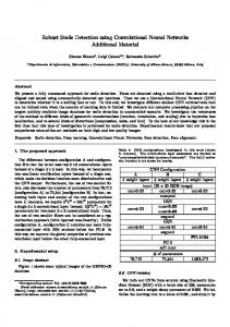
Robustness of Stochastic While Stochastic’s neural tissue will always look different every time it is grown because of the stochastic nature of neuronal splitting, it always forms a processing network that correctly computed the NAND function. This confers some robustness to the phenotype of the network in spite of the stochastic, but genetically directed, growth process. However, the developmental process is far more robust than that. For example, we can manually kill (remove) neurons of a fully developed tissue and have a similar functional (but somewhat scarred) tissue grow back. Fig 4 shows an example where we even removed the tissue seed CPT, which has an important role in the organisms development (without its external signal, glial cells of type ACPT0 do not proliferate). While the morphology of the self-repaired tissue has changed, it still computes the NAND function. More than

Figure 4: Robustness of Stochastic under cell death. Half the neural tissue from Fig. 3 was removed (left). After 80 time steps a different, but functional tissue arises (right).

anything, this observation helps illustrate the potential capabilities of developmental processes in artificial chemistries to create robust information processing neural tissues even under the breakdown of part of their structure. Note that the self-repair property of Stochastic was not evolved (or even hand-coded), but rather emerged as a property of the developmental process. Naturally, these robustness traits can be augmented and exploited under suitable evolutionary pressures.

Figure 5: Evolution objective: to double the functionality of the original organism.

very different in both structure and algorithm. The simplest, Stochastic A, evolved the fastest with the more straightforward morphology (Fig. 6). Its genome is short (Fig. 7) when compared to evolved organisms in other runs, but is substantially more difficult to understand compared to its ancestor.

Evolution of organisms in Norgev Here, we present the evolutionary capabilities of Norgev, that is, how its genetic structure and chemistry model allow for the evolution of developmental neural networks that solve pre-specified tasks. In the previous section we presented the Stochastic organism, which grew into a neural tissue that computed a NAND function on its inputs. Our goal was to study how difficult it would be to double the tissue’s functionality and compute a double NAND on three inputs, and send the result to two outputs (Fig. 5). Because one of the mutational operators used in the Genetic Algorithm is gene doubling (see Astor and Adami, 2000), we surmised that there was an easy route through duplication and subsequent differentiation. Because of the universality of NAND, showing that more complex tissues can evolve from Stochastic suggests that arbitrary computational tissues can evolve in Norgev. The input signal was applied for four time steps (the time for the input to pass through the tissue and reach the output), andp then P the output was2 evaluated by a reward function R = 1− i (yi (x) − ti (x)) where x is the input, y the tissue’s output, and t the expected output. Organisms were then selected according to a fitness function given by the average reward over 400 time steps, and a small pressure for small genome sizes and neuron numbers. Mutation rates were high and evolution was mainly asexual. Details of the experiments will appear elsewhere (Hampton and Adami, in preparation). We evolved organisms that obtained the double NAND functionality in two separate runs on massively parallel cluster computers, over several weeks. The two solutions were

Figure 6: Stochastic A neural tissue expressing 6 different cell types. Most of the axonal connections that spread out from the central sensor are not utilized. Instead, the actual computation takes place in a compact area near the center. After careful analysis of the genome, paired with an evaluation of the physical connections present in the neural tissue, we came to the conclusion that the organism had not reused any genomic material to double the NAND function, but had instead completely rewritten its code to implement a shorter and more efficient algorithm when compared to the ancestor we wrote. Let us embark once again in a quick step-by-step genome analysis. Gene 1 is active in the tissue seed, which then splits off a cell of type ACPT0 and APT2. After this, the gene is forever shut off because of the repressive NNY(apt2) condition. Cell ACPT0 then splits off cells of type ACPT1, ACPT2 and ACPT3 through gene 2. This gene is always active, and thus ACPT0 cells are always in an inhibitive activation state (due to action atom INH1). Gene 6 makes ACPT1 cells grow a dendrite to sensor SPT0 and have

1. 2. 6. 7. 8. 10. 11.

MUL(cpt) NNY(apt2) SUB(ep2) SUP(acpt0) SUB(spt3) SUB(ep2) SUP(acpt1) ANY(spt0) ADD(cpt) MUL(NT1) ADD(acpt2) SUP(acpt2) NAND(spt1) NSUP(spt1) ADD(acpt0) SUP(acpt3) ANY(apt0) NAND(eNT) OR(ep2) ANY(acpt3) NSUP(acpt3) MUL(acpt1) NAND(NT2) AND(acpt0) NNY(rfp)

⇒ ⇒ ⇒ ⇒ ⇒ ⇒ ⇒

SPL(acpt0) SPL(apt2) GRA(ep2) DFN(NT1) SPL(acpt2) SPL(acpt1) INH1 GRA(acpt5) MOD-(NT1) SPL(acpt3) GDR(spt0) SPL(acpt1) GRA(ep2) GRA(acpt5) MOD-(NT1) GDR(spt1) DFN(NT2) GRA(ep2) GRA(apt1) GDR(acpt1) GDR(acpt2) GRA(apt0) EXT0 PRD(ip0) DFN(eNT) INH1 MOD-(NT1) GRA(apt0)

Figure 7: Genome of evolved Stochastic A organism. Gene numbering is maintained from the ancestral genome, and gene 11 is a new gene which was randomly created. Gene atoms in light gray appear to be useless and are considered “junk”.

same-type daughter cells. These are the cells that cover the whole substrate in Fig. 6. Gene 7 causes ACPT2 cells to grow a dendrite towards sensor SPT1, an axon towards actuator APT1 and define its neurotransmitter as NT2. Through gene 8, ACPT3 cells grow a dendrite to sensor SPT2, a dendrite to cells ACPT2, and an axon to actuator APT1. Gene 11 is the most cryptic. This gene is only active in the first ∼3 time steps of the organism’s life, and effectively makes cells of type ACTP0, ACPT1 (only the ones in the center, not all the rest) and ACPT2 grow an axon towards the actuator APT0. Once the tissue has developed, gene 10 is used by all cells for processing sensory information (neurotransmitter eNT), on which it performs a NOT function.

gene 10 is used for neural processing once the tissue has developed, and it thus has a structure more conducive to further function doubling.

Figure 9: The computation carried out by Stochastic A.

Figure 8: Effective neural circuit grown by Stochastic A. Dashed axonal connections grow due to gene 11, which is only active during the first moments of the organisms life. Axons and neurons that have no influence on the final computations are rendered in light gray. The effective neural circuit is shown in Fig. 8. The result is processed in three time steps instead of the incorrectly postulated minimum of four time steps. This is due to an implicit OR function computed by the actuator cells that we did not anticipate, but which was discovered and exploited by the organism. The neural tissue is applying a NOT function at a relay of its inputs, and then an OR on the actuators to arrive at the double NAND (Fig. 9). The resulting simplicity of the organism is apparent from the fact that only

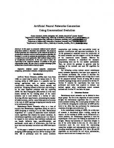
Another organism that solved the problem was Stochastic B, which took considerably longer to evolve, and that turned out to be highly complex and difficult to understand. In Fig. 10, cellular structures can clearly be seen in which stripe-like patterns of two different neural types succeed one another. These stripes were different for each organism, and reflect a stochastic development. The axonal connections linking all these neurons are so interwoven that it is difficult to believe that this organism is actually acting on its inputs instead of undergoing some recurrent neuronal oscillation. We were unable to describe the development and internal workings of this organism due to its complexity. However, a complete description is in principle always possible because of our access to all of the organism’s internal state variables, and more importantly, to its genetic code: the source of its dynamics. Taking the first steps in that direction, we studied the neuronal activation under each of the eight possible input configurations (Fig. 10). We can clearly see neuronal activity that follows the striped pattern on the right-hand side of the tissue (for inputs of the form x0x → 11). Remarkably, the left side of the tissue does not follow the same organization and thus we theorize that although they have the same cell type, they have differentiated internally even further depending on their position on the tissue. We came to the conclusion that this organism is not performing the same internal computation as Stochastic A. We can see this by inspecting input 110 → 01, and noticing that no tissue neurons are activated, and thus there is no neuron performing the NOT

000 → 11

001 → 11

010 → 11

011 → 10

100 → 11

101 → 11

110 → 01

111 → 00

Figure 10: Neuronal activity of a Stochastic B neural tissue under the eight possible binary input combinations, where active neurons are shaded, and inactive neurons white. This activity only reflects neurotransmitters that will be injected by active neurons down their axonal branches.

function on the last input.

Conclusions Biology baffles us with the development of even seemingly simple organisms. We have yet to recreate insect neural brains that perform such feats as flight control. As an even simpler organism, the flatworm C. elegans, has a nervous system which consists of 302 neurons, highly interconnected in a specific (and mostly known) pattern, and 52 glial cells, but whose exact function we still do not understand. Within Norgev, we have shown that such structural biocomplexity can arise in silico, with dendritic connection patterns surprisingly similar to the seemingly random patterns seen in C. elegans. And we might have been baffled at the mechanism of development and function of our in silico neural tissue if it were not for our ability to probe every single neuron, study every neurotransmitter or developmental transcription factor, and isolate every part of the system to understand its behavior. Thus, we believe that evolving neural networks under a developmental paradigm is a promising avenue for the creation and understanding of robust and complex computational systems that, in the future, can serve as the nervous systems of autonomous robots and rovers.

Acknowledgements Part of this work was carried out at the Jet Propulsion Laboratory, California Institute of Technology, supported by the Physical Sciences Division of the National Aeronautics and Space Administration’s Office of Biological and Physical Research, and by the National Science Foundation under grant DEB-9981397. Evolution experiments were carried out on a OSX-based Apple computer cluster at JPL.

References Astor, J. and Adami, C. (2000). A developmental model for the evolution of artificial neural networks. Artificial Life, 6:189–218. Belew, R. R. (1993). Interposing an ontogenetic model between genetic algorithms and neural networks. In NIPS5 ed J Cowan (San Mateo), CA: Morgan Kaufmann. Dittrich, P., Ziegler, J., and Banzhaf, W. (2001). Artificial chemistries–A review. Artificial Life, 7:225–275. Eggenberger, P. (1997). Creation of neural networks based on developmental and evolutionary principles. In Proc. ICANN’97, Lausanne, Switzerland, October 8-10, 1997. Gruau, F. (1995). Automatic definition of modular neural networks. Adaptive Behaviour, 3:151–183. Kirschner, M. and Gerhart, J. (1998). Evolvability. Proc. Natl. Acad. Sci. USA, 95:8420–8427. Kitano, K. (1990). Designing neural network using genetic algorithm with graph generation system. Complex Systems, 4:461–476. Koza, J. R., Keane, M. A., and Streeter, M. J. (2003). The importance of reuse and development in evolvable hardware. In 5th NASA/DoD Workshop on Evolvable Hardware, Chicago, IL, USA. IEEE Computer Society. Koza, J. R. and Rice, J. P. (1991). Genetic generation of both the weights and architecture for a neural network. IEEE Intl. Joint Conf. on Neural Networks, 2:397–404. Nolfi, S. and Parisi, D. (1995). Evolving artificial neural networks that develop in time. In Advances in Artificial Life, Proceedings of the Third European Conference on Artificial Life, pages 353–367. Springer.