PHYSICAL REVIEW E 77, 056105 共2008兲
Evolution of weighted scale-free networks in empirical data Y.-H. Eom, C. Jeon, and H. Jeong* Department of Physics, Korea Advanced Institute of Science and Technology, 305-701 Daejon, Korea
B. Kahng Department of Physics and Astronomy and Center for Theoretical Physics, Seoul National University, 151-747 Seoul, Korea 共Received 14 September 2007; published 16 May 2008兲 Weighted scale-free networks exhibit two types of degree-strength relationship: linear and nonlinear relationships between them. To understand the mechanism underlying such empirical relationships, theoretical evolution models for weighted scale-free networks have been introduced for each case. However, those models have not yet been tested with empirical data. In this study, we collect temporal records of several online bulletin board systems and a movie actor network. We measure the growth rates of degree and strength of each vertex and weight of each edge within the framework of preferential attachment 共PA兲. We also measure the probability of creating new edges between unconnected pairs of vertices. Then, based on the measured rates, linear and nonlinear growth models are constructed. We find that indeed the dynamics of creating new edges and adding weight to existing edges in a nonlocal manner is essential to reproduce the nonlinear degreestrength relationship. We also find that the degree-driven PA rule is more appropriate to real systems rather than the strength-driven one used for the linear model. DOI: 10.1103/PhysRevE.77.056105
PACS number共s兲: 89.75.⫺k, 89.65.⫺s
I. INTRODUCTION
The Barabási and Albert 共BA兲 model 关1兴, recently introduced for scale-free 共SF兲 networks, is a distinct model compared with the random graph 关2兴, the small-world model 关3兴, and the static model 关4兴, in the perspective that the network is evolving, i.e., the total number of vertices increases with time. In the BA model, the preferential attachment 共PA兲 rule was introduced, where a new vertex is attached to existing vertices with the probability linearly proportional to the degree of the target vertices. Later, the PA rule was justified using the empirical data of the coauthorship network 关5兴. These pioneering studies were limited to binary networks and were later extended to weighted networks in order to model real networks. For example, the coauthorship network contains edges with weights that represent the number of papers written together between two coauthors. The dialogue network of an online bulletin board system 共BBS兲 has edge weight, which is the frequency of dialogues between two people. The edge weight in the worldwide airport network is the number of passengers traveling between two cities. In such weighted networks, strength si, defined as the sum of weights on the edges connected to a given vertex i, is a physical quantity that is as important as the degree ki. In general, strength and degree are related to each other in a nonlinear fashion, si ⬃ ki 关6–11兴. The exponent can be either 1 共called the linear case兲 or not 共called the nonlinear case兲, depending on the systems. The linear and nonlinear cases have been found in the scientific coauthorship network and the worldwide airport network, respectively 关6兴. The linear case was modeled by Barrat, Barthelemy, and Vespignani 共BBV兲 关12兴. The BBV model is generally similar
*
[email protected] 1539-3755/2008/77共5兲/056105共7兲
to the BA model, however, they are different in that the PA rule is applied to the strength instead of the degree in the BBV model. Hereafter, the former 共latter兲 PA rule is called the strength-driven 共degree-driven兲 PA. Once a new connection is made, the updating of the edge weight is followed locally at the edges connected to the target vertex. This local updating rule yields a linear relationship between the degree and strength. On the contrary, it was suggested that the nonlinear relationship can be achieved by the nonlocal updating of the edge weight 关13兴. This idea has been embodied in a few evolution models 关14,15兴. In the model proposed by Bianconi 关14兴 共Wang et al. 关15兴兲, a target vertex is selected by the degree-driven 共strength-driven兲 PA rule. Moreover, the edge weight is strengthened or reinforced at selected internal edges for both models. However, the dynamics of a new connection of edges between existing, but as yet unconnected vertices was not taken into account. While the two models are successful in generating a nonlinear relationship between the degree and strength, they have not yet been tested with empirical data. In this paper, we test the elements proposed in the two above-mentioned papers with empirical data. For this purpose, we measure the key quantities that drive the evolution of weighted networks from the empirical data, which are the growth rates of the degree and strength of each vertex, and the weight of each edge as a function of time, i.e., the total number of vertices. Indeed, we find that the nonlocal updating of the edge weight is an important element in obtaining the nonlinear relationship between the degree and strength. Moreover, based on the obtained results, we modify the previous model to include the case where the total number of edges increases nonlinearly with respect to the number of vertices. We find that the result obtained from the degree-driven PA rule can fit better with the empirical data, and the dynamics of adding edges between unconnected pairs of vertices must be taken into account.
056105-1
©2008 The American Physical Society
PHYSICAL REVIEW E 77, 056105 共2008兲
EOM et al.
TABLE I. Summary of the statistics of the evolution of network structure for the weighted networks. ⌬ is the temporal resolution of the data. T is the period for observation. Other quantities are defined in the text.
Size ⌬ T p q r ␣1 ␣2 ␣3
Loco
Bar
Google
Movie
7435 1 day 1670 days 0.51⫾ 0.01 0.0068⫾ 0.0005 0.0017⫾ 0.0001 1.12⫾ 0.002 1.85⫾ 0.008 2.28⫾ 0.009
3988 1 day 1575 days 0.82⫾ 0.01 0.026⫾ 0.001 0.11⫾ 0.01 1.07⫾ 0.001 1.70⫾ 0.005 1.81⫾ 0.012
39918 1 day 1259 days 0.84⫾ 0.01 0.66⫾ 0.02 0.084⫾ 0.006 1.04⫾ 0.002 0.99⫾ 0.004 0.84⫾ 0.01
752682 1 year 117 years 0.01⫾ 0.002 0.00084⫾ 0.00028 0.016⫾ 0.007 1.61⫾ 0.02 1.85⫾ 0.04 1.55⫾ 0.05
II. ANALYSIS OF EMPIRICAL DATA
Our data set is comprised of four real networks, three BBSs 共loco, bar, and Google兲 关16,17兴, and movie actor networks 关18兴. A BBS is an online social communication system where users post messages and others reply to them. The BBS data contain the information of user names in the from and to fields and the posting date of each message. This yields a weighted network where vertices are users and a pair of users is connected if the users exchange at least one message. The weight wij of the edge between two users i and j is determined as the number of messages they communicate. The movie data include information on movie titles, actors, and production years. In this network, the vertices are actors and the edges between two actors i and j are connected if they act in the same movie. The weight wij between the vertices i and j is the number of co-starring movies. The strength si of a vertex i is defined by si = 兺 j苸nn共i兲wij, where nn共i兲 is the nearest neighbor of the vertex i. For the BBS 共loco and bar兲 networks, the strength distributions exhibit heavy-tailed behaviors, which were also shown in our previous works 关17兴. Other networks show similar behaviors. Table I shows the summary of the structural features of the weighted networks. We examine the evolution pattern of the weighted networks in the real world, particularly focusing on the three evolution processes 共Fig. 1兲: 共i兲 Addition of a new vertex: A new vertex is introduced and edges are created from the new vertex to the existing vertices. ⌸ext denotes the probability of connecting edge to the vertex. This process is regarded as an occurrence during a unit time interval. 共ii兲 Creation of internal edges: Internal edges are created between existing vertices that are unconnected. ⌸int is the probability of connecting the two vertices. 共iii兲 Reinforcement of edge weight: The weights of the selected existing edges are increased by a unit weight. Both processes 共i兲 and 共iii兲 are proposed in Refs. 关14,15兴, but 共ii兲 is introduced here. To be specific, the number of vertices at a given instant is regarded as time t. Let Lext共t兲, Lint共t兲, and Wrei共t兲 be the numbers of edges at time t created from processes 共i兲–共iii兲, respectively. Empirical measurements show that these quan-
tities increase in power law as Lext共t兲 ⬇ pt␣1, Lint共t兲 ⬇ qt␣2, and Wrei共t兲 ⬇ rt␣3 asymptotically. p, q, and r are constants, and the exponents ␣1, ␣2, and ␣3 vary depending on the systems, as listed in Table I. For all networks, ␣2 and ␣3 are nontrivial, indicating that the internal activity in the form of creating internal edges and strengthening edge weights is not negligible in BBS networks. It is noteworthy that these exponents are larger than 1 for the loco, bar BBS, and movie actor networks, indicating that these systems become more densely connected with an increasing time; this is called accelerated growth. For the Google BBS network, however, the exponents ␣1 and ␣2 are close to 1, suggesting a linear growth. The exponent ␣3 is less than 1. To understand the evolution mechanism microscopically, we measure the increasing rates of each quantity, and obtain kernels ⌸ that drive the dynamics for each evolution process 共i兲–共iii兲. The kernel function ⌸ determines the attachment probability for topological growth and the probability of weight increase for link weight reinforcement. For the degree growth resulting from adding new vertices, the kernel function is reduced to that of preferential attachment. The function ⌸ext共k兲 is described by (a)
(b)
k
n
i
n
j
(c) n
j
Πext
i
j (d)
k
Πint
k
i
n
k
Πrei i j
FIG. 1. 共Color online兲 Schematic illustration of the evolution dynamics of a weighted network. 共a兲 Initial configuration. 共b兲 A new vertex n is introduced to the system and connects to an existing vertex i with probability ⌸ext 共external growth兲. 共c兲 Two existing vertices k and j that are still unconnected are connected with probability ⌸int 共internal growth兲. 共d兲 Edge weight between existing vertices i and j is increased by one with probability ⌸rei 共edgeweight reinforcement兲.
056105-2
EVOLUTION OF WEIGHTED SCALE-FREE NETWORKS IN …
PHYSICAL REVIEW E 77, 056105 共2008兲
TABLE II. Numerical values of the exponents defined in the kernels.
0.94⫾ 0.08 0.64⫾ 0.05 0.83⫾ 0.08 0.41⫾ 0.02 0.87⫾ 0.08
1.25⫾ 0.13 0.77⫾ 0.09 0.67⫾ 0.1 0.27⫾ 0.04 0.87⫾ 0.09
1.36⫾ 0.14 1.14⫾ 0.09 0.70⫾ 0.08 0.62⫾ 0.08 1.40⫾ 0.07
0.64⫾ 0.06 0.62⫾ 0.06 0.50⫾ 0.03 0.48⫾ 0.03 1.01⫾ 0.08
(a)
-2
10
xi=ki xi=si
10
-6 0
10
n共k,t兲
dki = m1⌸ext,s共si兲. dt
共3兲
It was found that ⌸ext,s共si兲 ⬃ si1,s with 1,s ⬇ 0.64 for the loco BBS network. The measured values of the exponents 1,k and 1,s for other systems are listed in Table II. The increasing rate of quantity kij, which is the average number of links newly connected between unconnected vertices i and j, is measured as a function of kik j, dkij = m2⌸int,k共kik j兲, dt
共4兲
and measured as a function of sis j, dkij = m2⌸int,s共sis j兲, dt
2
10
10
4
6
10
8
6
10
8
10
sisj ,kikj
(c) rei
0
(d)
-2
10
-4
10
0
10
2
10
xij=kikj xij=sisj
-4
10
xij=wij
-6
4
10
0
10
w
2
10
10
4
10
sisj ,kikj
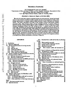
FIG. 2. 共Color online兲 Cumulative functions of the kernels defined in Eqs. 共2兲–共4兲 as functions of their argument for the loco BBS network. 共a兲 ⌸ext for the process 共i兲. 共b兲 ⌸int for the process 共ii兲. 共c兲 ⌸rei as a function of weight wij for the process 共iii兲. The straight lines are guidelines with slopes of 1.87 共d兲 ⌸rei as functions of kik j or sis j. The dashed lines are guides to the eye showing slope 1.
共2兲
where m1 = 具dLext / dt典 is the average number of edges attached from a new vertex during a unit time interval. 具¯典 is the average over different times. It was found that ⌸ext,k共ki兲 ⬃ ki1,k with 1,k ⬇ 0.94 for the loco BBS network. The increasing rate of degree ki can also be measured as a function of strength,
10
Π
(c)
dki = m1⌸ext,k共ki兲, dt
0
10
(c)
-2
10
共1兲
where ⌬ki is the number of new links that attach to vertex i with degree k during ⌬t, and n共k , t兲 is the number of vertices with degree k at time t. Because of the data fluctuation, we use a time-average kernel function. That is, ⌸ext = 具⌸ext共k , t兲典. The increasing rate of degree ki of a vertex i by the attachment of a new edge from a new vertex is measured as follows:
6
10
10
Π
⬇ C共t兲k ,
4
10
xij=kikj xij=sisj
-8
10
s,k
rei
⌸ext共k,t兲 =
2
10
10-6
0
10
兺i ⌬ki
-4
10
-4
10
(b)
10
(c) int
Movie
0
-2
Π
Google
(c)
ext
1,k 1,s 2,k 2,s 3,w
Bar
Π
Loco
10
100
dwij = m3⌸rei共wij兲, dt
共6兲
where m3 = 具dWrei / dt典 is the average number of reinforced weights during a unit time interval. It was found that ⌸rei共wij兲 ⬃ wij3,w with 3,w ⬇ 0.87 for the loco BBS network. The measured values of the exponents 3,w for other systems are listed in Table II. Notice that to calculate ⌸ext,k共ki兲, we calculate the increment of the degree ⌬kext i 共兲 of each vertex i at a given instant using only the connection from an introduced vertex. If the total number of edges generated from the new vertex at a given instant is ⌬Lext共兲, then ⌸ext,k共ki , 兲 = ⌬kext i 共兲 / ⌬Lext共兲. Since we are interested in the degree dependence of the kernel ⌸ext,k共ki兲, we take the average over time and vertex indices with the same degree. To reduce the noise level, we use the cumulative function defined as ⌸共c兲共x兲 = −兰⬁x ⌸共y兲dy, as shown in Fig. 2. The other kernels ⌸ext, ⌸int, and ⌸rei are determined in the same manner and shown in Figs. 2共a兲–2共c兲, respectively. We found that ⌸rei共wij兲 is almost independent of kik j and sis j in Fig. 2共d兲 共c兲 共x兲 ⬃ x, which corresponds to ⌸rei共x兲 since it follows ⌸rei = const. The numerical results suggest that a relationship between the degree and strength exists in the form of s ⬃ k with ⬇ 1.4 for the loco BBS network. Thus, 1,k ⯝ 1,s and 2,k ⯝ 22,s.
共5兲
where m2 = 具dLint / dt典 is the average number of internal edges attached between unconnected vertices during a unit time interval. It was found that ⌸int,k共kik j兲 ⬃ 共kik j兲2,k with 2,k ⬇ 0.83 and ⌸int,s共sis j兲 ⬃ 共sis j兲2,s with 2,s ⬇ 0.41 for the loco BBS network. The measured values of the exponents 2,k and 2,s for other systems are listed in Table II. The increasing rate of edge weight wij is
III. LINEAR GROWTH MODEL
Based on the numerical data, we construct a linear growth model for the weighted network, where the total numbers of vertices and edges linearly increase with time. This case can be seen in the Google BBS network. The dynamic rule for the model is as follows: 共i兲 At each time step, a new vertex is introduced into the system and it attaches ᐉ1 edges to the
056105-3
PHYSICAL REVIEW E 77, 056105 共2008兲
EOM et al. 0
existing vertices selected by the linear PA rule applying to the degree. The target vertices are selected with the probability linearly proportional to their degrees. Here, we use the degree-driven PA rule only to solve the problem analytically. A minimal weight w0 = 1 is assigned to each new edge. 共ii兲 At the same time, ᐉ2 edges are created between those numbers of unconnected pairs of existing vertices i and j, selected with a probability linearly proportional to the product of their degrees, i.e., kik j. 共iii兲 ᐉ3 existing edges are selected and their weights are increased by w0. The selection is made following the linear PA rule applied to the weight wij. The above rules are repeated until there are N vertices in the system. This linear growth model enables us to understand the dynamic process analytically. The dynamic equation for processes 共i兲 and 共ii兲 is given as 关19兴
ki ki = 共ᐉ1 + 2ᐉ2兲 , t 兺 kj
共7兲
j
where 兺 jk j is given by 2共ᐉ1 + ᐉ2兲t. The solution is given as ki共t兲 = ᐉ1共t/ti兲1 ,
共8兲
where 1 = 共ᐉ1 + 2ᐉ2兲 / 2共ᐉ1 + ᐉ2兲 and ti is the time at which vertex i was introduced into the system. The dynamic equation for process 共iii兲 is
wij = 2ᐉ3w0 t
wij
兺 wm,m⬘
共9兲
.
m,m⬘
Then, the solution is wij = w0共t/ti,j兲2 ,
共10兲
where the exponent 2 = ᐉ3 / 共ᐉ1 + ᐉ2 + ᐉ3兲 and ti,j is the time at which the edge 共i , j兲 is created. Combining Eqs. 共7兲 and 共10兲, the dynamic equation for the strength evolution is written as
si wij ki = 兺 + t j苸nn共i兲 t t
=2ᐉ3w0
兺 j苸nn共i兲
wij
兺 wm,m⬘
共11兲
+
ki t
共12兲
m,m⬘
=
ᐉ1 + 2ᐉ2 ᐉ3 si + ᐉ1共t/ti兲1 . 共ᐉ1 + ᐉ2 + ᐉ3兲t 2共ᐉ1 + ᐉ2兲t
共13兲
10
冦
if 1 ⬎ 2 ,
si ⬀ ki ln ki if 1 = 2 , ki2/1 if 1 ⬍ 2 .
10
-6
10
-8
(b)
-4
10
10-6
Google Minimal 0
10
1
10
-8
2
10
3
10
4
10
10
10
Google Minimal 0
1
10
2
10
0
s
P(w)
10-6
10
104
(c)
10-4
-10
Google Minimal
100
101
102
w
10
10
3
k
10-2
10-8
2
10
s 100
103
104
100
(d)
Google Minimal 101
102
103
104
k
FIG. 3. 共Color online兲 The distributions of several physical quantities—strength 共a兲, degree 共b兲, weight 共c兲 for the Google BBS 共red square with solid line兲—and the comparison with those obtained from the linear model 共black square with solid line兲. The degree-strength relationship is also compared 共d兲. The numerical data are averaged over 30 network configurations with the same size as N = 39 918 of the Google BBS.
Consequently, the model generates a degree-strength relationship that is linear when 1 ⬎ 2, but nonlinear when 1 ⬍ 2. The above result is reduced to that of the model introduced by Bianconi 关14兴 where step 共ii兲, the creation of new internal links, is ignored, i.e., ᐉ2 = 0. Further, the selection rule for step 共iii兲 is slightly different. In Ref. 关14兴, once a vertex is chosen with the probability proportional to its strength ⌸i = si / 兺 js j, then its partner for connection is chosen with a probability proportional to its weight ⌸ij = wij / 兺ᐉwiᐉ, where the index ᐉ is the nearest neighbor of i. However, in the proposed model, we choose target edges with the probability given by Eq. 共9兲. However, the two methods reduce to the same result. Next, using the relation ␥ = 1 + 1 / previously derived in Ref. 关20兴 for the linear kernel case, we obtain the exponents associated with the power-law decaying behaviors of the degree and edge-weight distributions. They are obtained as ␥k = 2 + ᐉ1 / 共ᐉ1 + 2ᐉ2兲 and ␥w = 2 + 共ᐉ1 + ᐉ2兲 / ᐉ3, respectively. Then the exponent associated with the power-law decaying behavior of the strength distribution is obtained using Eq. 共14兲 as ␥s = ␥k when 1 ⬎ 2 and ␥s = ␥w when 1 ⬍ 2. We compare the analytic results with the empirical data obtained from the Google BBS network, of which ␣1 ⬇ ␣2 ⬇ 1. Even though the kernels of ⌸ext and ⌸int for the Google BBS depend nonlinearly on the degree and the product of the degrees, the analytic solutions fit well with the empirical results, as shown in Fig. 3.
We find that in a long time limit ki
-4
0
10-2
P(k)
P(s)
10-2 10
10
(a)
IV. NONLINEAR GROWTH MODEL
冧
共14兲
Here, we study the nonlinear evolution case where the total number of edges increases nonlinearly as a function of the total number of vertices. We use the degree-driven and strength-driven PA rules, with the respective measured val-
056105-4
EVOLUTION OF WEIGHTED SCALE-FREE NETWORKS IN …
PHYSICAL REVIEW E 77, 056105 共2008兲
ues of 共1,k, 2,k兲 and 共1,s , 2,s兲 of the loco BBS network in Table II, and compare the respective results with the empirical data. The growth of the network starts from an initial configuration composed of N0 = 10 vertices, which are sparsely connected, for example, forming a ring, allowing for internal edge connections at a later stage. Otherwise, the internal edge growth becomes trivial. Each edge has a preassigned weight w0 = 1. The network evolves under three evolution dynamics: 共i兲 the addition of a new vertex and its connection to the existing vertices, 共ii兲 the creation of internal edges, and 共iii兲 the reinforcement of the weights of existing edges. For steps 共i兲 and 共ii兲, degree-driven and strength-driven PA rules are applied, respectively. Thus, two types of networks result. To be specific, the construct rules are as follows: 共i兲 At each time step, a new vertex is introduced in the system. Depending on time step t, the number of edges emanating from the new vertex varies as ᐉ1共t兲 = pt␣1 − p共t − 1兲␣1. p and ␣1 are chosen from Table I in order to compare the resulting network with the empirical data. The target vertex i for each edge is chosen with the probability, ⌸ext共x1,i兲 =
1 x1,i
兺j x1,j
,
1
共15兲
where x1,i can be ki 共si兲 for the degree-driven 共strengthdriven兲 case. Then, 1 is given as 1,k and 1,s in Table II, respectively. The initial weight of each new edge is given as w0 = 1. This process reflects the dialogues between the new user and the existing users. 共ii兲 ᐉ2共t兲 = qt␣2 − q共t − 1兲␣2 edges are created between unconnected pairs of vertices, where q and ␣2 are given in Table I. The pair of target vertices for each edge is chosen with the probability ⌸int共x2,ij兲 =
2 x2,ij
x2,ij 兺 i,j
,
2
共16兲
where x2,ij is kik j 共sis j兲 for the degree-driven 共strengthdriven兲 case. Correspondingly, 2 is 2,k and 2,s adopted from Table II, respectively. The addition of multiple edges to the same pair of vertices is not allowed. The weight of each new edge is also given as w0 = 1. This process reflects the dialogues between the existing users who have not exchanged any messages previously. 共iii兲 ᐉ3共t兲 = rt␣3 − r共t − 1兲␣3 edges are chosen from all connected pairs of vertices with the probability given below, and their weights are strengthened by w0 = 1. r and ␣3 are given in Table I. The probability is given as ⌸rei共wij兲 =
wij3
wij 兺 i,j
3
,
共17兲
where 3 is given in Table II. Multiple additions of edge weights to the same pair are allowed in this process. This process reflects the additional message exchange between users who have exchanged messages previously.
P(s)
0
10-1 10-2 10-3 10-4 10-5 10-6 10-7 10 0 10
loco K-Model S-Model
1
10
2
10
P(w)
P(k)
0
10 -1 10 10-2 -3 10 -4 10 -5 10 100 100 10-1 10-2 10-3 10-4 10-5 10-6 10-7 100
s
10
3
10
4
10
5
loco K-Model S-Model
101
k
102
103
loco K-Model S-Model
101
102
w
103
104
FIG. 4. 共Color online兲 The distribution of several quantities— strength 共a兲, degree 共b兲, and weight 共c兲 for the loco BBS network. The empirical data 共red square with solid line兲 are compared with the results obtained from the models with the degree-driven 共solid line兲 and the strength-driven 共dotted line兲 PA rule. The simulation data are averaged over 30 network configurations of the same size of the loco N = 7435.
This nonlinear model is reduced to the linear model when ␣1 = ␣2 = ␣3 = 1 and 1 = 2 = 3 = 1 for the degree-driven case only. Numerical simulations were performed with the measured parameters listed in Tables I and II for the loco BBS network and the other networks. The results of the degree, strength, and edge weight distribution for the model network are shown in Fig. 4, where the degree-driven 共strengthdriven兲 case is denoted by a solid line 共dotted line兲. The strength and edge-weight distributions obtained from the simulations are in good agreement with the empirical data for the loco BBS network, but the degree distributions obtained from the model based on both the degree-driven and strength-driven PA slightly deviate from the corresponding empirical one. We examined the degree-strength relationship s ⬃ k 关6–11兴 for the model network in Fig. 5共a兲 and compared it with the empirical data obtained from the loco BBS network. The two versions of the model network exhibit different values of . The degree-based model, i.e., with the degreedriven PA rule, produces a closer value k ⬇ 1.56 to the value loco ⬇ 1.40 obtained from the loco BBS network than the value s ⬇ 1.81 obtained from the strength-based model. In addition, we calculated the confidence interval using the bootstrap procedure to compare the measured values of from the empirical data, the degree based model, and strength based model. The 95% confidence interval of for the loco BBS data runs from 1.36 to 1.43. Those obtained from the degree-based and the strength-based models run
056105-5
PHYSICAL REVIEW E 77, 056105 共2008兲
EOM et al. 105
100
104
Y(k)
103
s 100 100
V. CONCLUSION
10-1
102 101
than the strength-based model for reproducing the structural features of BBS networks.
loco K-Model S-Model
loco K-Model S-Model 101
k
102
103
10-2 100
101
k
102
103
FIG. 5. 共Color online兲 The degree-strength relationship 共a兲. The data are obtained from the empirical data 共circle兲, the degree-driven model 共solid line兲, and the strength-driven model 共dotted line兲. The weight heterogeneity as a function of degree 共b兲. The data are obtained from the empirical data 共circle兲, the degree-driven model 共solid line兲, and the strength-driven model 共dotted line兲. The simulation data are averaged over 30 network configurations of the same size as that of the loco N = 7435.
from 1.52 to 1.59, and from 1.76 to 1.86, respectively. This result supports our conclusion that the degree-based model fit better than the strength-based model to reproduce the empirical result. We also examined the heterogeneity of the weights on the edges connected to a given vertex introduced in Refs. 关21–23兴. We measured Y 2i = 兺 j共wij / si兲2 ⬃ k−i 关21兴. If the weights are homogeneous, then it would be Y 2i ⬃ 1 / ki. If a dominant edge with weight wi,j ⬃ si exists, then Y 2i ⬃ O共1兲. As shown in Fig. 5共b兲, the empirical data of the weight heterogeneity for the loco network is more closely reproduced by the degree-based model than by the strength-based model as loco ⬇ 0.66, k ⬇ 0.66, and s ⬇ 0.50. We obtained a 95% confidence interval of for the loco BBS data that runs from 0.63 to 0.70 from the empirical loco data using the bootstrap procedure. This range is close to that 关0.65,0.68兴 obtained from the degree-based model, but deviates from that 关0.48,0.52兴 obtained using the strength-based model. The results for other BBS networks showed similar behaviors. Therefore, we conclude that the degree-based model is better
关1兴 A.-L. Barabási and R. Albert, Science 286, 509 共1999兲. 关2兴 P. Erdös and A. Rényi, Publ. Math. Inst. Hung., Acad Sci. 5, 17 共1960兲. 关3兴 D. J. Watts and S. H. Strogatz, Nature 共London兲 393, 440 共1998兲. 关4兴 K.-I. Goh, B. Kahng, and D. Kim, Phys. Rev. Lett. 87, 278701 共2001兲. 关5兴 H. Jeong, Z. Neda, and A.-L. Barabasi, Europhys. Lett. 61, 567 共2003兲. 关6兴 A. Barrat, M. Bathelemy, R. Pastor-Satorras, and A. Vespignani, Proc. Natl. Acad. Sci. U.S.A. 101, 3747 共2004兲. 关7兴 J.-P. Onnela, J. Saramaki, J. Hyvonen, G. Szab, M. de Menezes, K. Kaski, A.-L. Barabási, and J. Kertész, New J. Phys. 9, 179 共2007兲. 关8兴 A. de Montis, M. Barthelemy, A. Chessa, and A. Vespignani, Environ. Plan. B: Plan. Des. 34, 905 共2007兲.
We have analyzed the evolution records of real weighted BBS networks to understand the growth mechanism of weighted networks. We measured the growth rates of the degree and strength of each vertex and the weight of each edge as a function of time, that is, the total number of vertices. Based on the measured results, we constructed two evolving weighted network models. The models had three common elements: 共i兲 The addition of new vertices, 共ii兲 the addition of new internal edges between two previously unconnected vertices, and 共iii兲 the strengthening of weights on existing edges. Processes 共ii兲 and 共iii兲 were applied independently of 共i兲, so that the dynamics arising on the edges occurred in a nonlocal manner. In processes 共i兲 and 共ii兲, the degree-driven PA rule performs better than the strengthdriven PA rule in reproducing the features of real systems as a rule of choosing target vertices. Depending on the ratio between the growth rates of the numbers of vertices and edges, we established linear and nonlinear growth models. The Google BBS network can be reproduced using the linear growth model and the other two BBS networks and movie actor network can be reproduced through the nonlinear growth models. Our study is meaningful from the perspective that the existing concepts and models for weighted networks are tested with empirical data. We find that the existing models are overall successful in reproducing the empirical results; however, the nonlinear growth model must be used to match the empirical results. ACKNOWLEDGMENTS
This work was supported by Acceleration Research CNRC of MOST/KOSEF 共H.J., B.K.兲 and Grant No. R012005-000-1112-0 共Y.-H.E., C.J.兲 from Korea Science and Engineering Foundation 共KOSEF兲.
关9兴 S. Valverde, G. Theraulaz, J. Gautrais, V. Fourcassie, and R. V. Sole, e-print arXiv:physics/0602003, IEEE Intell. Syst. 关10兴 S. Valverde and R. V. Sole, Phys. Rev. E 76, 046118 共2007兲. 关11兴 Q. Ou, Y.-D. Jin, T. Zhou, B.-H. Wang, and B.-Q. Yin, Phys. Rev. E 75, 021102 共2007兲. 关12兴 A. Barrat, M. Barthelemy, and A. Vespignani, Phys. Rev. Lett. 92, 228701 共2004兲. 关13兴 K.-I. Goh, B. Kahng, and D. Kim, Phys. Rev. E 72, 017103 共2005兲. 关14兴 G. Bianconi, Europhys. Lett. 71, 1029 共2005兲. 关15兴 W.-X. Wang, B.-H. Wang, B. Hu, G. Yan, and Q. Ou, Phys. Rev. Lett. 94, 188702 共2005兲. 关16兴 loco.kaist.ac, kr: bar.kaist.ac.kr: http://bbs.keyhole.com 关17兴 K.-I. Goh, Y.-H. Eom, H. Jeong, B. Kahng, and D. Kim, Phys. Rev. E 73, 066123 共2006兲. 关18兴 http://www.imdb.com
056105-6
EVOLUTION OF WEIGHTED SCALE-FREE NETWORKS IN … 关19兴 S. N. Dorogovtsev and J. F. F. Mendes, Europhys. Lett. 52, 33 共2000兲. 关20兴 S. N. Dorogovtsev, J. F. F. Mendes, and A. N. Samukhin, Phys. Rev. Lett. 85, 4633 共2000兲. 关21兴 M. Barthelemy, A. Barrat, R. Pastor-Satorras, and A. Vespig-
PHYSICAL REVIEW E 77, 056105 共2008兲 nani, Physica A 346, 34 共2005兲. 关22兴 E. Almaas, B. Kovacs, T. Vicsek, Z. N. Oltvai, and A.-L. Barabasi, Nature 共London兲 427, 839 共2004兲. 关23兴 S. H. Lee, P. J. Kim, and H. Jeong 共unpublished兲.
056105-7