Evolution operator equations: Integration with

RIVISTA DEL NUOVO CIMENTO

VOL. 20, N. 2

1997

Evolution operator equations: integration with algebraic and finitedifference methods. Applications to physical problems in classical and quantum mechanics and quantum field theory G. DATTOLI(1), p. L. OTTAVIANI(2), A. TORRE (1) and L. VJ~ZQUEZ(3)

(1) ENEA, Dipartimento Innovazione, Settore di Fisica Applicata, Centro Ricerche Frascati via E. Fermi 45, 00044 Frascati, Roma, Italy (2) ENEA, Dipartimento Innovazione, Settore di Fisica Applicata, Centro Ricerche Bologna via Don Fiammelli 2, 40129 Bologna, Italy (~) Departamento de Matemdtica Aplicada, Escuela Superior de Informdtica U',~iversidad Complutense - 28040 Madrid, Spain (ricevuto il 6 Maggio 1997)

2 4 9 18 23 27 35 37 43 45 49 51 52 56 6O 65 68 81 85 89 99 102 102 103 104

Part I 1.1. 1.2. 1.3. 1.4. 1.5. 1.6. 1.7. 1.8.

Introduction Preliminary considerations on exponential operators More about the formalism of exponential operators Hermite polynomials and exponential operators Hermite polynomials with many indices and exponential operators Different realizations of the Heisenberg group Matrix representation and operatorial ordering Evolution problems in classical and quantum mechanics: the case of linear and quadratic potentials The fractional Fourier transform

1.9. Part II Introduction II.l. The problem II.2. II.3. Symplectic integrators II.3.1. First-order integrators II.3.2. Higher-order symplectic integrators II.3.3. Symmetric second-order integrators Liouville equation and differencing schemes II.4. II.5. Quantum mechanics and unitary integrators Higher-order symmetric integrators II.6. Geometrical light optics and differencing schemes II.7. II.8. Particle optics and differencing schemes II.8.1. Fokker-Planck equation and finite difference schemes Part I I I III.1. Introduction One-dimensional motion of a particle in a potential III.2. III.2.1. Newtonian mechanics III.2.2. Quantum mechanics

9 Societ6 Italiana di Fisica

1

4

G. DATTOLI, P. L. OTTAVIANI, A. TORRE and L. V~ZQUEZ

1.2. - P r e l i m i n a r y considerations on e x p o n e n t i a l operators

In this section we deal with the formalism of the exponential operators, which are the most commonly used operators to treat evolution problems. We establish the rules relevant to the action of an exponential operator on a given function and the rules for the disentanglement of exponential operators. The first example we discuss is provided by the so called shift or translation operator e ~(d/dx), where ~t is a parameter. It is well known that its action on a function of x produces a shift of the variable by )~, namely (I.2.1)

e~(a/dx)f(x) : ~

]~n a n

~

)n

n=O n--~. dx n f ( x ) = n=o -~.. f ( n ) ( x ) = f ( x + ,~).

To derive eq. (I.2.1) we have made the requirement, assumed valid for all the exponential operators we will deal with, that e ~(d/d~) can be expanded in Taylor series and f ( x ) is continuous and infinitely differentiable. The apparent trivial operatorial identity (I.2.1) can be exploited to state other important identities as that relevant to the dilatation operator, namely (I.2.2)

e ~x('t/d~)f ( x ) = f ( e ~ x) .

The fact that eq. (I.2.2) is just a consequence of the identity (I.2.1) is easily understood if we perform the following change of variable: (I.2.3)

x = e ~.

The 1.h.s. of eq. (I.2.2) can therefore be written as (I.2.4a)

e Zx(d/dx)f ( x ) = e Z(d/dO)f ( e 0).

From the identity (I.2.1) it follows that (I.2.4b)

e ~l(d/dO)f ( e 0) = f ( e o +~) = f ( e ~ x ) .

By using the same method of variable substitution we can prove other important identities, as e.g. the relation (I.2.5)

e~2(a/d~) f ( x ) = f

x

1

;

ix I < ~ '

which also follows from (I.2.1). In fact, by replacing x with 1/~ in the 1.h.s. of eq. (I.2.5), we find (I.2.6a)

e -)4d/d~)

1

1

x

which can be easily generalized as (I.2.6b) elxn(d/dx) f(x) = f

( _

x

n - ~ / 1 - 2(n - 1)

) X n-1

by means of the change of variable x = ~ - 1~/1/~.

ix IO,

i

t~h n

--,nE0 - - H ~ ,

n(x, Y),

A=ae-b2>~O.

The polynomials H~, n(x, y) satisfy the recurrences a ~x H~. n(X, y) = amHm_ 1, ~(x, y) + bnHm, n -

1 (X,

y),

(I.5.4b)

a-~-Hm, n(X, y) = bmHm_l,~(x, y) + cnH,~,~ l(x, y) ay and can be explicitly constructed through the Rodrigues-type formula (I.5Ac)

Hm, n(x, y) = ~m + n 1 = ( - 1 ) m + n e x p -~(ax 2 + 2 bxy + cy e) -ax - e"~ x 3y p [ -'~2 ( a x 2 + 2 b x y + c y 2 )

].

Along with the H,~, n(x, y) one can introduce the adjoint denoted by G~. ~(x, y) and specified by the generating function (I.5.5a)

[

exp ux + v y -

l(cu

] u vn

- 2buv + av 2) =

--Gm

m,n=0

n(X, Y),

re!n!

and by the recurrences (I.5.5b)

{ff-ff~G,n,n(X,y)=mGm_l,n(X,y),

3

--Gm, n(X, y) = nGm,~_l(X, y). 3y

Furthermore the analog of (I.5.4c) writes (I.5.5c)

Gin, ~(x, y) =

=(-1)~+~exp

[1

- ~ exp - ~ (c~2-2b~rl+a~ 2) -9-~-~-~

]

(c~ 2 - 2b~] + ay 2) ,

where (I.5.5d)

~ = ax + by,

~] = bx + cy .

Further properties of the above polynomials will be discussed within the framework of the theory of generalized harmonic-oscillator eigenfunctions.


26

It is now worth stressing that Kamp~ de Feriet-type polynomials can be introduced in this case too, by using the generating functions

(I.5.6a)

t

e (ax+by)t+(bx+cy)h+z(at2+2bth+ch)=

~'~

~

~ Z exp]ux+vy+--(eu2-2buv+av2)]= L

--(:I)

~~ t~h~ ~

m,n=O m . nY. I

A

~,

m n U

(X ~

, v,

z)

mv n

- - - - Wm ~(X, Y, Z)" m,n=O m!n! '

J

The polynomials Ore, n and qJm, n are easily expressed in terms of Hm, ~ and Gin,~ as follows:

r

- i V x~

n(x, Y, z) = im+n(2z)(m+n)/2Hm,~

' -i ~ Y ) '

(I.5.6b)

qlm n(X, Y,

,

m,n[[--i

X--v~, - i - ~ z z )

and it is clear that eqs. (I.5.6b) are the generalization of eq. (I.4.9b). By exploiting the recurrences of Hm, n(X, y) and G~, ~(x, y), it can be shown that r n(X, Y, Z) and qJm, ~(x, y, z) satisfy the generalized heat equation

(I.5.6c)

f

A~zqlm, n ( X , y , z ) = { - ~ X 2 - 2 b -ax- 3y -~z O m ' n ( x ' y ' z ) =

c~

~

aa~----~

+ a-~y 2 } U k l m 'n ( X , Y ' Z) '

$~ay +c

r

n(X,y,z).

The importance of this last result is evident. We can conclude indeed that qlm,~(x, y, z) = e x p [ A \ ax 2 - 2 b (I.5.6d) ~)m,n(X,

ax ay

y, z ) = e x p [ z ( a ~ - ~ + 2 5

+ a-~y 2

-~-

qJ,~,n(x, y, O), Om, n(X ,

O)

Furthermore, since

{

Wm,~(x, Y, 0) = xmy n,

(I.5.7a)

1

Om, n(x, y, O) = x'~y '~ = A m+n (c~ - b~7)m(a~ -

b~)n,

we can obtain the following relation: (I.5.7b)

[l(c

Hm, n(X, y) = exp - - ~ -

~

- 2b--

axgy + a ~ y 2

thus leading, for f(x, y) = ~ am, nxmy n, to ~'~ n

(I.5.7c)

exp --~ c - - 2b-+a 9x 2 3x 3y

5)]

f(x, y) = ~ a,~, nq~,~, n(x, y, z).

EVOLUTION OPERATOR EQUATIONS: INTEGRATION WITH ALGEBRAIC ETC.

27

However, a further important operatorial identity we should emphasize is provided by (I.5.7d)

exp

z ( 82 a2 -~ c--Sx2 - 2b--Sx 8y + a

f(x, y) =

= f (x + 2z -ff~ , y + 2z 8--~--) exp [ -~ Z C--sxifi2 - 2b sxS~Sy +a~/~ )], with

8~

-

A

c--

8x

-

8y

,

8~]

-

,(

A

a - -

8y

-

8x

.

The interested reader is addressed to refs. [15] for further comments on the properties of the multi-index Hermite polynomials.

1.6.

-

Different

realizations

of

the

Heisenberg

group

In sect. 1.2 we have shown that, by using a proper variable transformation, the action of exponential operators, containing first derivatives, can be reduced to that of displacement-like operators. Such a result should be reconsidered, because, in spite of its apparent simplicity, may lead to surprisingly interesting consequences. The operators ~ and ~ are said to provide a one-parameter realization of the Heisenberg group if they satisfy the commutation bracket [~, ~ ] = i

(I.6.1)

and if 1 commutes with both ~ and ~ . The simplest realization of the group is given by the so-called Bargman representation, namely d P - dx '

(I.6.2)

m = x.

By using the identifications (I.6.3)

d ~ = x--, dx

~ = In (x),

we obtain a less trivial realization of the Weyl group, being indeed [~, ~ ] = 1. Furthermore, by noting that if eq. (I.6.3) holds we find (I.6.4)

~(lnx)n=n(lnx) n-l,

~ ( l n x ) n= (lnx) n+l,

we can conclude that (ln x) n is a quasi-mononial under the action of the operators (I.6.3). A straightforward by-product of this last observation is that eigenvalue problems formulated by using the realization (I.6.2) of the Heisenberg group can be rewritten in terms of the operators (I.6.3) and viceversa.


28

The Bessel eigenvalue problem is a particularly appropriate example. In terms of the realization (I.6.3) it writes d

[x ~x (x ~ ) + e21~ - n2l Jn(x) = O ,

(I.6.5a) while its

isospectral counterpart in the representation (I.6.2) reads -~

(I.6.5b)

+ e 2~ - n 2 J~(e ~ = O.

According to the above considerations we can also conclude that

d-~-II(lnx)~=H~(lnx'y) dx ]J

[ (d-~x exp y Xdx

(I.6.6a) and (7)

[(

(I.6.6b)

d

d

exp y x dx

dx

)]

x, ~ m=o --H,~(lnx, y) m!

and finally (s)

I (I.6r :)

exp

~

nm

d x -~x d /I1J f(x) = ~n an~=o--~.Hm(lnx, y (x [ ~x = Y)"

if f ( x ) = E a ~ x "~.

n Analogous considerations can be developed if we realize the Heisenberg group as

(I.6.7)

~ = (x - b) 2 - - , d dx

m=--

1 (x - b)

(7) By H.(lnx, y) we denote the Kamp~-de Feriet polynomials obtained by replacing x with In x. (s) It should also be noted that by setting x = e ~ we have

d2 exp y ~ -

]

e n,~-_

~

m=0

ymn2m

m[ -enO = eYn2xn'

and hence

exp[y(x-Xdx although its convergence is not ensured for any y.

n=O

29


In this case it is easily understood that 1/(x - b ) n is the relevant quasi-monomial. By using this representation, the Bessel equation may be written as (b = 0) (I.6.8)

x4

d2

d

+ 2 x 3 -d-x +

e

-2/x_

n 2

/

]

-1/x)

=Hn

(1)

Furthermore, it is also easily understood that (I.6.9)

[(

exp y x 4 + 2x 8dx 2 dx

--

xn

= O.

Jn(e

,y

9

We could provide an almost infinite number of examples of different realizations of the Heisenberg group. However, according to the discussion of the present section and to that of sect. 1.2, we can conclude that a fairly general representation may be provided by

(I.6.10)

io = f ( x ) ~ x '

m = ~ f(x')

"

Needless to say the associated quasi-monomials are F ( x ) = relevant Bessel equation reads (I.6.11)

fxdx'/f(x')

and the

d2 d -+ f ( x ) f ' (x) - - + e 2F-l(x) - n 2} J n ( e F l(x)) = 0 . f2(x) dx 2 dx

It is now worth pointing out that we can take advantage of the previously discussed realization of the Weyl group to construct more complicated groups. The generators of S U ( 1 , 1) can be, e.g., realized as

K+ =

(I.6.12)

F2(x)

1[

h'-

1 d2 2 f2(x) dx 2

h'0= ~ l + 2 F ( x ) f ( x ) ~

d dx

.

The usefulness of these last results will be commented later in the paper. We have so far discussed representations of the Weyl group based on Bargmantype realizations. As it is well known the Weyl group can be realized by using the formalism associated to the creation ~ § and annihilation ~ operators, satisfying the relati,m (I.6.13)

[~, ~ § = 1,

~ § a = n,

where ~ is the number operator. The action of ~ and ~ § on the Fock space, spanned by the eigenvectors In} of the number operators ~, is specified by (I.6.14)

~]n)=n]n),

~ln) = V ~ l n -

1),

~+ In) = V ~ + 1 I n + 1}.

30

G. DATTOLI, P. L. OTTAVIANI, A. TORRE

and L. V)tZQUEZ

As is also well known the differential realization of ~ and ~ + is provided by (I.6.15)

x d ~ = - + -2 dx '

x 2

~+-

d dx

The vectors In} in the x-representation are provided by the harmonic-oscillator eigenfunctions (I.6.16)

1

Hen(X) exp [ - l x 2 ] ,

(xln) - un(x) - 4h/~~

the Hermite polynomials Hen being defined in (I.4.1)-(I.4.2). Furthermore, from the last of eq. (I.6.14) it also follows that Un(X) satisfy the eigenvalue equation (I.6.17)

(d2

- - - -dx 2 +

lxz

)

u~(x) =

(1) n

+

~

u,~(x) .

Even though the formalism of creation-annihilation operators is well known and widely exploited it is less known that a similar formalism is associated to generalized harmonic-oscillator eigenfunctions constructed in terms of the generalized Hermite polynomials Hm, n(X, y) and Gm, n(X, y). We note indeed that according to the formalism of sect. 1.5 we can introduce the following operators:

al, + =

8 8x

(ax + by)

(I.6.18a) l(ca

gl,-

8)

b ay

x

2

and a

&e, + =

( bx + cy )

8y

(I.6.18b) .

&a, -

.

.

A

.

.

8x

a--

8y

+--

2

which satisfy the commutation relations (I.6.19)

[~, -, ~s, +] = 5r,~

(r, s = 1, 2)

and create and annihilate photons according to

(I.6.20a)

{

al, + Im, n} =~/-m-7 l i r a + 1, n), a2, + Im, n} = V n + l l m , n + 1}

EVOLUTION OPERATOR EQUATIONS: INTEGRATIONWITH ALGEBRAICETC.

31

and

51,- [m,

n) = V ~ [ m - 1, n), 52, Im, n) = V ~ l m , n - 1).

(I.6.20b)

The vectors Ira, n) are realized in the (x, y) configuration by (I.6.21)

(x, ylm, n)=~-~,n(x,y)- -4V~ ~ Hm,~(x,y)~ exp [ - ~-1z_TMz]

where M denotes the symmetric 2 x 2 matrix: M =

and _z the column vector:

The creation-annihilation operators (I.6.18) acting on the entangled Foek space [m, n) are not Hermitian conjugate to each other. For this reason we consider their Hermitian conjugates reported below x

51,+=

A~ ax

ay)

(I.6.22a)

2

1

-~ (ax+by)+ 3_

al,-

dx

and

+

(I.6.22b)

A ~ ax

3y

2'

A 1 a a2, - = ~ (bx + cy)- - - , $y

which act on the vectors Ira, n) in the same way as 51, • and ~ , _. act on Ira, n). Furthermore, it can be easily verified that ar, • = S r , ~ , r = 1, 2. The (x, y)-representation of the vectors Im, n) is provided by (I.6.23)

(x, ylm, n~=~m n(x,y)- 4V~ Gm'n(M~Z-)exp[-lzrMz]. '

~

h / m ! n!

4 -

-

It is easy to prove the orthogonality relation (I.6.24)

f dx ~ - cJr

d y e r , s(X, y ) "~m, n( x , Y) = (~m, vf~n,s

- oo

which allows to state that the entangled oscillator eigenfunctions ~m,n(x, y) and ~m, n(x, y) provide a biorthogonal system. By introducing the number operators { m - - 51, + 51, - ,

(I.6.25)

n = 52, + 5z, _,

m - - 51, + al, - ,

n = 52, + a2, _,

32

G. DATTOLI,P. L. OTTAVIANI,A. TORRE and L. VAZQUEZ

we can prove that :~V~,,~(x, y) and ~m,~(x, y) are eigenvectors of the hermitian operators m + n and ~ + ~ respectively, and hence they satisfy the same differential equation (I.6.26)

-

+ --zTMz

8x ' t31a

,/

4

Fr~ n(X, Y) = '

= (m + n + 1)

F,,,, ,~(x, y)

with Fm, n(X, y) denoting 9V,~, ~(x, y) and ~m, n( x, Y). Within this framework the operator

(I.6.27)

/

\ 8 / 8 y ] = --A c--Sx2 - 2b--Sx 8y + a

8x ' 8y

should be viewed as a generalized Laplaceoper~or. It is also worth stressing that the operators (al, +, a l , - ) , (a2, +, ~z, ), (51, +, 51, _), (a2, +, a2,-) provide a nonHermitian realization of the Weyl group. It is worth stressing that the SU(1, 1) group can be realized in terms of entangled differential operators as follows (9): (I.6.28)

h:+ = - - - zi - DT~ 18~, .2

A = -i- z V M - z , K_

-

2-

h'o = I ( z T S ~ + S T z ) . 2

-

In the following we will see that the above realization can be conveniently used to solve multidimensional SchrSdinger equations. Before closing this section we want to touch another important property of the creation-annihilation operators, namely their invariance under Fourier transform. As it is well known (see also sect. 1.9), the ordinary harmonic oscillator eigenfunctions are also eigenfunctions of the Fourier transform (FT) operator. The corresponding properties of the entangled harmonic-oscillator eigenfunctions are less known and will be discussed below. We define the bidimensional FT of -~Vm,n(X, y) as (I.6.29a) d ~ ( : ~ . , n(X, y) ) = cr

or

+ ~y)] = ~,. ,~(Q, ~), --~

oo

while the corresponding antitransform reads oo

'ss

(I.6.29b1 Jt'-l(~7~m,n(e, ~))~--- - ~

(3) Note that 8T = (8/8x, a/Sy).

do

d ~ . , , n ( O , ~)exp

(ex+~y)

]

9

EVOLUTIONOPERATOREQUATIONS."INTEGRATIONWITHALGEBRAICETC.

33

The ordinary FT operational rules can be generalized as follows: [ ~--~ (~'(.9Vm, ~(x, y))) = :gVm,n(X, y), O"

(I.6.30a)

~(Sz~Vm,,~(x, Y) ) = i26r(~Vm, n(x , Y) ) , 5-(zgV ..... (x, y) ) = 2i8, ~(~Vm n(x, y) ) ,

where (I.6.30b)

-

-

\3/3q

It is now straightforward to prove that in the Fourier space eq. (I.6.26) writes (I.6.31)

[-8.M3,,+ '-4

]

o'TM 1(7 ~ . , n ( _ a ) = ( m + n + l ) ~ , ~ , ~ ( _ a ) .

It is evident that eqs. (I.6.26) and (I.6.31) are structurally equivalent, apart from the interchange M-1___>~ of the matrix in the scalar products. The bidimensional FT of $'m, ,(X, y) will be defined according to (I.6.29a) as (I.6.32)

-~.~, ~(0, ~) = ~

'ss

dx

-~

dy ~m, ~(x, y) exp - ~ (0x + ~Y)

-r162

]

and it can checked that it satisfies eq. (I.6.31) as well. The biorthogonality property is preserved in the Fourier space too and in fact we get (I.6.33)

f de I d~.~r,s(O, - c~ - ac

~)~-m,n(O, ~)----(~m,r(~n,s"

The explicit forms of ~,~, ~(0, ~) and -~m, ~(0, ~) write

(-i)'t+ (1.6.34)

n

Hm,~(~-lo) exp[

~,~ ,,(o, ~ ) - 4v~ ~

( -i)m+n -~m, n(0, ~) -- 4 V ~ f ~

_ [

1oTM-I_~]

-~_ 1 o~T~-I ]

Gin, n(O)_ exp - -4 -

,

-q '

Let us now discuss how the creation-annihilation operators transform in the Fourier space. This aspect of the problem is more conveniently understood if we introduce the following definitions: (I.6.35a)

~+= ~2,

i z- z,

--

=

=

a2,

--Z

2-

-~ M - 1 3

z

34

G. DATTOLI, P. L. OTTAVIANI,A. TORRE and L. V~ZQUEZ

and

(I.6.35b)

~+

al, + : ! Z__ ~ _ l ~z,

-

=

2,

~_

_

_

(tl,

1

:

= ~ z + a ~ .

+

It is also worth stressing that (I.6.35c)

~ = (~_)t,

~_ = (~+)t.

By using eqs. (I.6.30) we obtain the important relations (I.6.36a)

~ ( A_ + )

=

~_+ ~

i

-

a + i M S.o ,

2-

.

.~'-(A_) . --JC_ = /

-

--

-la+igo

2

and (I.6.36b) ~'(B+) _

=

~+

= !M-l(7-i~o, 2 -

~ - ( B_ - )

= ~--

= - a +i i M S o . A 2-

-

It is important to stress that the definition of bidimensional FT is not unique. We can indeed introduce the following generalization: Qr

ar

i

(I.6.37)

~-@

(f(x,

y) ) -

TA

-~z

where Q is a symmetric 2 x 2 matrix: Q = ~)T, AQ its determinant and generic 2-variable function. In this case we obtain

f(x,

y)is

a

9~(~)n(_~ ) --

(I.6.38) ~em, A g ) -

( - - i ) m+n ~ Q

Gm, n(~_a) exp[

l aTQM-1Qa_]

and the analogous of (I.6.31) write by replacing _M with MQ -i Before closing this section we want to discuss a final example of creationannihilation operators, which can be defined as (I.6.39a)

~_

)

Vm

+x ,

a+ = ~

[

x

1

m m- 1

The Hermitian conjugate of the above operators are provided by -

Vm

- - -

dx

+x

,

~$=

x

-

-

m m- 1

dx

x)


35

and it is evident that ~_ and ~§ are hermitian conjugate to each other only for the case m = 2. The operators ~_ and ~+ satisfy the rule of commutation (I.6.40)

[~_, ~+ ] = 1

and act as ordinary annihilation-creation operators on the function (I.6A1)

q~'~)(x)- ~ 1

H(~m)(x, - 1 ) exp - -~- ,

which, accordingly, is shown to be an eigenfunction of the operator g§ g_, namely (I.6.42a)

g+

n~(m)(x)

a _ q~m)(x) =

or, in differential representation (I.6.42b)

X-~x +

ram_-----~ ~

+x

~O(nm)(x)= n q ~ ) ( x ) .

In this section we have presented a fairly general approach to the theory of Weyl group and to the harmonic-oscillator eigenfunetions. Most of the concepts developed here will be exploited in the forthcoming part of the paper.

1.7. - Matrix representation and operatorial ordering

In sect. 1.3 we have seen that the ordering problem (I.3.10a) relevant to the operator

[[

U(2) - exp 2 ax

+ flY -~x + ~ y ay

3x

is reduced to the system of first-order differential equations (I.3.10b), which in matrix form reads (I.7.1)

- ~ [y(,~)]

a

[y(,~)]"

As a consequence, U(;t) can be cast in the form (I.7.2)

U()~) = e ~ ,

U(0) = 1,

where H denotes the matrix on the r.h.s, of eq. (I.7.1). By keeping the derivative of both sides of eq. (I.7.2) with respect to )[ we obtain (I.7.3)

- d- ~(2) = HU(2), d~

U(0) = i .


36

The operator H can be therefore considered the matrix representation of the operator at the argument of the exponential in U(;t), namely

H-

aX--ay +ZYTx + 7

Y -~y -

ax

- x - -

Since we have obtained the correspondence

(I.7.4)

a x - -ay +fly

+7

- x - -3x

---*

,

we can attempt the following identifications:

(I.7.5)

-----> x Oy 1

,

y

-~x

--~

'

--

Y ay

-

x - -

---~

ax

0

,

which provide a realization of differential operators in terms of Pauli matrices. The identifications (I.7.5) is unambiguous since the Pauli matrices yield a basis for 2 x 2 matrices. More in general, independently of the specific realization, we can use the minimal representation for the angular momentum generators, namely

:),

(I.7.6)

:), 1(1 :) o

"

We can draw a fairly important consequence from these apparently trivial results. Let us therefore consider the following problem:

(I.7.7)

i

d~

d~

= [a(Z) J_ + fl(;t) J+ + 2i7(;t) J0] ~f,

where a, fi, 7 are )~-dependent functions. Since the operator in eq. (I.7.7) does not commute with itself at different 2, we cannot perform a straightforward integration of eq. (I.7.7). This is indeed a genuine problem of time ordering. We can overcome this trouble by using the matrix realization of the angular momentum operators. Equation (I.7.3) is indeed still valid even though H is an explicitly ;t-dependent matrix. Moreover, assuming for U an ordered form of the type (I.3.6), according to the matrix representation (I.7.6), we find

(I.7.8)

{ e-~/2 U(~.) = e -i~(~).?_ e -ib(~)2+ e c(~)?o= ~ae -c/~

beC/2 I ( 1 + ab) e ~/2]'

where the ordering functions a, b and c are specified by eq. (I.7.3).


37

It is interesting to note that by setting

(I.7.9)

(D(2) U(2) = \B(2)

A(2)/, C(;O] !

we obtain that each column of the above matrix satisfies the same differential equations, namely

(I.7.10)

d---~-A=-~A+flC, d~

A(0) = O,

d C=aA+7C, d~

C(0)

1

and similarly for the entries D and B, except that the appropriate initial values are D(0) = 1, B(0) = 0. After some manipulations we find for C (I.7.11)

d2 1 da d { 7 da + --~d7 _ fl a _ y 2) C = O ~d~---:C - a d~ d;t C + / --ad~--

which specifies the 2-dependence of the function C. Similar equations can be obtained for A~ B, D. The characteristic functions (a, b, c) of the ordering procedure (I.7.8) are then obtained in terms of the A, B, C functions (10). The procedure we have described is essentially the Wei-Norman time ordering method [16] according to the point of view of refs. [17].

1.8. - Evolution problems in classical and quantum mechanics: the case of linear and quadratic potentials

An evolution problem in classical mechanics may be solved by using different methods. The choice of the method is just matter of convenience and depends on the problem under study. The evolution of an ensemble of non-interacting particles, driven by a given potential, may be treated by using the Liouville equation, which accounts for the evolution of the phase space density distribution. The problem could also be treated by solving the Hamilton equations of motion for each particle. We consider the following one-dimensional Hamiltonian: p2

(I.8.1)

H(q, p) =

2m

+ V(q),

where V(q) is an unspecified potential and p, q are canonical variables, in the sense that their Poisson bracket is equal to unity, namely (I.8.2a)

{q, p} = 1.

(10) The knowledge of D is redundant since the determinant of the matrices (I.7.8)-(I.7.9) is equal to unity.


38

We remind that in general {f(q, p), g(q, p)} -

(I.8.2b)

afag

8fag

8q 8p

8p 8q

The Liouville equation associated to the Hamiltonian (I.8.1) writes [18] (I.8.3)

-~o(q, P; t) = {H, Q} =

+

m 8q

(q)

o(q, P; t),

where V' (q) ~ (d/dq) V(q) and Q(q, p; t) is the particle density distribution in the ( q - p) phase space. The formal solution of eq. (I.8.3) can be cast in the form (I.8.4)

Q(q,p;t)=exp[(

p 8 + V' (q) 3 ) t ] f(q, p), m 8q -~p

with f(q, p) being the particle distribution at t = 0. The operator (I.8.5)

UL(q,p;t)=exp[(

p 8 +V'(q) 8 ) ]t m 8q -~p

can be considered as the classical evolution operator associated to the Liouville equation (I.8.3). As is also well known, the Hamilton equations of motion can be written as (I.8.6)

=-{H,q}=

P,

ib=-V'(q).

m

If we denote by z the vector (I.8.7) and if we use the notation [19] (I.8.8)

:f:_

8f 8 8q 8p

8]" 8 8p 8q

we can write the formal solution of the Hamilton equations as (I.8.9)

z(t)

=e

-:H:tz

and we can interpret (I.8.10)

UH(q, P; t)

----e - : H : t

as the evolution operator associated to the Hamilton problem (I.8.1). Before entering into further details, relevant to the operator ordering techniques applied to the formalism of the evolution operator for classical problems, we exploit the methods developed in the previous section to solve eqs. (I.8.3) and (I.8.9), when V(q) is a linear potential, namely (I.8.11)

V(q) = mgq ,


39

where g is a constant. In this case we find for ~) the following expression:

[/ (I.8.12)

Q(q, p; t ) = e x p | | [\

a)]

p8 + mg -~p t f( q, p ) = m 8q = e x p [ l g t 2 ~q ]eXp[mgt ff_~]exp[

=f q- Ptm

pt 8 m 8q ] f(q' p) = 1 t2 , p + m g t ). ~g

From the above result we can easily obtain the equation of motion for the average values of q and p. By noting in fact that or

oo

f dq f dpo(q, p; t)-- X

(I.8.13a) and

(I.8.13b)

q(t)- f dq f dpq~(q, p; t),

p(t)-

f dq f dppq~(q, p; t)

we find (I.8.14)

q(t) = qo + pm t

21 gt2'

p(t)

Po mgt,

which are nothing but the free-falling body equations, (q0, Po) denoting the initial values. The solution of eq. (I.8.6) can be written in the form (I.8.15)

[(

z(t)=exp -

a)]

p 8 +rng m Sq ~p

t z

-'

which yields strightforwardly the result (I.8.14). Let us now consider the quantum counterpart of the above problem, which in the SchrSdinger picture writes (I.8.16)

ih

~f =

2m 8q 2

)

+ mgq ~f .

By assuming that initially ~ is provided by a Gaussian, namely (I.8.17)

1

~f(q) - ~r

exp -

G. DATTOLI, P. L. 0TTAVIANI, A. TORRE and L. VMZQUEZ

40

and by using eq. (I.3.42c) we find that the time evolution of the probability amplitude is (I.8.18)

oq ~(q, t) - 4 V ~

-exp

a~ + i2c ct/2

_ gt 2 2~ct

6 2cc

(~______L_ q ( q + (1/2) gt 2 exp - i 2 2 c c t oqz + i)cc ct/2

q-

'

where 2c = h / m c is the Compton wavelength and c is the velocity of light. It is evident that the characteristic feature of the first part of the motion is a significant broadening of the initial packet. Another problem which can be treated exactly, within a classical or quantum framework, is that relevant to the quadratic potential. We consider indeed an Hamiltonian of the type p2 1 H = - - + - k ( t ) q2, 2 2

(I.8.19)

where k is assumed as a time dependent function and the mass of the particle is taken as m = 1. The Liouville equation associated to (I.8.19) is (I.8.20)

3--tQ(q' p; t) =

-p-~q +k(t)qff--~}o(q,p;t)

9

By noting that the differential operators appearing on the r.h.s, of eq. (I.8.20) can be embedded to form the algebra (I.8.21)

J+ = - q ~3p ,

J_ = - p ~ q3q ,

(

~0 = ~1 q-~q 3 -P ~p

,

we can use the Wei-Norman method to write the solution of eq. (I.8.20) in the form

o(q, P; t)

(I.8.22)

= e u+(t)2§

e u (t)3 e2U3(t)Jof ( q , p).

By using the identities discussed in the previous section we end up with

o(q, P; t) =f(q(t), p(t) ) ,

(I.8.23) where (I.8.24)

p(t)]

- u + (t) e -~3(t)

e -u3(t)

]

According to (I.8.2~ and the matrix representation (I.7.6), it is easy to realize that the evolution operator UL in eq. (I.8.22) satisfies the equation (I.8.25)

d

- - UL(t) = dt

(::)

UL(t);

AUL(O) = 1.


41

It is important to emphasize that the determinant of U is 1 at any time, this implies that (I.8.26)

{q(t), p(t)} = 1

for any t and thus U acts as a canonical transformation. The Wei-Norman procedure can also be applied to the Lie series method and this aspect of the formalism will be discussed below. Before considering this evolution problem from the Lie series point of view, let us specify the initial distribution to the Gaussian case

f(q'P)= 2z ~

(I.8.27)

1

exp

[-- !' Z- T~-I(0) 2 Z]

where ,E(0) is the fluctuation matrix, namely

l !

In this ease we find that the evolution of the distribution is specified by { (I.8.29)

o(q,p;t)=

1 [ 1 ] ~=___~ exp - - z Tg: i(t)_z , 2 z ~v/det 2(0 ) 2-

[~(t)] -1 = ULT(t)[~(0)] -1UL(t). Sometimes the matrix Z(0) is written in terms of the Twiss parameters (fl, a, ?), namely

;)

(I.8.30)

The Twiss parameters are assumed to satisfy the relation (I.8.31)

fly-a2=1,

so that (I.8.32)

(det E(0)) 1/2 = e.

This last quantity is an invariant of motion, as it follows from the fact that UL(t) has unit determinant, and is linked to the phase-space area. In particular (I.8.33)

A = ~e

in the language of accelerator physics is known as beam emittance. Let us now consider a slightly modified aspect of the Lie series method; we rewrite indeed the Hamiltonian (I.8.19) in the form (I.8.34)

H = l z T Hoz , 2-


42

where Ho is the Hamiltonian matrix specified by

( = :)

(i.s.35)

No =

.

The Heisenberg equations of motion can be rewritten as (I.8.a6)

-d - z = S--Hoz , dt-

where S is the so-called symplectic matrix, namely

satisfying the property (I.8.38) According to (I.8.36) we can write the evolution of the vector z in the form (I.S.39)

z_(t) =

~o(t

') dt

]}

z(0),

where the external braces denote time ordering, since we have assumed that the Hamiltonian (I.8.19) is explicitly time dependent and hence the matrix S H o does not commute with itself at different times. The ordering problem can be overcome by using the Pauli matrices and by rewriting S H o as A

A

(I.8.40)

~

~

SHo(t) = - k(t) ~ + + ~ _.

We can therefore apply the Wei-Norman procedure in this case too and thus obtain a result analogous to that already obtained and summarized by eqs. (I.8.23)-(I.8.24). The quantum evolution problem can be treated by solving the SchrSdinger equation (h = 1) (I.8.41)

i a- -

9t ~f =

[

1 Y

2 ~q2

+

1 k(t)

~

q2 ]

~f '

whose solution is easily obtained by recalling that the operators (I.4.42)

A i 2 K+= ~q ,

h:-=

i ~ 2 aq2,

1( a 1) h:0= 2 q ~ +-2

realize a S U ( 1 , 1) algebra. We can therefore write the evolution operator associated to (I.8.41) in the form (I.4.43)

U(t)

=

e ](t)[~+ e g(t)~- e 2h(t)R~


43

By using the matrix realization of the SU( 1, 1 ) group generators, which writes as

=(Oo :)

(I.8A4)

Oo) o= (lo Ol)

we find that the characteristic functions (g, h, f ) satisfy the differential equations

fi = -f' +2hg+l=0,

(I.8.45)

+f2+k(t)=O,

h(0) = 0 , g(0)=0, f(0) = 0.

Furthermore, by using the operational rules discussed in the previous section, we find (I.8.46)

~(q, t) = or

_

exp[-h/2] exp 2V~ _~ 2g

-h[(1 - f g )

+e

where ~(q', 0) represents the wave function at initial time.

1.9. - The fractional Fourier transform

In this section we will discuss the concept of fractional order Fourier transform (FOFT) to prove that it can be framed within the context of the so far developed formalism. As is well known, the harmonic-oscillator functions are eigenfunctions of the ordinary Fourier transform (FT) operator, which according to Namias [20] will be denoted by ~--~/2, namely (I.9.1)

~'-~/2 [e-x2/4He~(x)] =~o

=

1

2 V~_

!

e -x2/4Hen(X) e -i(xy/2)dx

=

e -~('/2)[e -x2/4Hen(X)],

with Hen(X) specified by (IA.2). The obvious generalization of (I.9.1) writes (I.9.2)

~r

= ein"[e-x2/4Hen(X)].

By denoting the FOFT ~'a operator by e i~, i.e. (I.9.3)

~-a = e i ~


44

and by keeping the derivative of both sides of eq. (I.9.2) with respect to a, we obtain the following differential realization for A: .4 = - ~d 2 + l x 2 - -1. dx 2 4 2

(1.9.4)

It is obvious that for a real the operator :~-, is unitary, as it follows from the hermiticity of A. It is also obvious that the action of ~ r on a given function of x can be viewed as that of an evolution operator associated to a quantum quadr~ic Hamiltonian [21]. According to the discussion of the previous sections, we can cast ~ r in the form

~ a = e -(i/2)a e)~a)fi,+eg(a)Y._ e 2h(a).~o

(I.9.5a)

with the functions g(a), h(a), f ( a ) explicitly given by (I.9.5b)

1 f ( a ) = - tan a , 2

g(a) = sin (2 a ) ,

e -ix(,) = cos a .

Finally, by using the identities discussed in the previous section, we easily get (I.9.6)

f(x) =

exp [ - i ((a/4) ~ + a / 2 )] 2 ~lsina

9exp

I

[ --

~x2tana 4

]!

d x ' f ( x ' ) exp ~

cosa

_

_

- - X

t

)2]

where ~ = sgn (a) and - z < a < ~. It is also easy to verify that for a = z / 2 the r.h.s, of (I.9.6) yields the ordinary FT as given in (I.9.1). In sect. 1.6 we have discussed the properies of the entangled harmonic-oscillator eigenfunctions under bidimensional FT. In this section we will discuss the concept of bidimensional FOFT. According to the discussion of the present section and to that of sect. 1.6, we can define the bidimensional FOFT operator as (I.9.7)

:~"a = e ia$,

__ ~ = _ oT ~ -1 az + 1 z T M z -- 1 . -

4

-

Using the SU(1, 1) realization provided by (I.6.28) and exploiting the operational rules e ~y~- ~l,(x, y) = e(i/2)~-T~-~y(x, y ) ,

e~~

y) = e~/2?(ef/2x, e~/2y),

e~R*~(x, y) -

dx'

dy'exp ---~(z-z')rM(z-z

') ~o(x', y ' ) ,


45

A

we can explicitly define the action of :~', on a given function F(x, y) as oo

(I.9.9)

~ar F(x, y) = e-i~-i(~/2)aV~ 4zlsinal

J dx' I dy'.

. . . .

"exP[ 4 c t n ( a ) [ z T M z - - z ' T M z '

COS2a zTMz']] F(x'' y')

with - z/2 < a < z/2. According to the discussions of the previous sections we can also prove further important properties of the type (I.9.10a)

:~", z~'~+ = e - i ~ ze i,~ = z cos a - 2i sin a M - 13z,

which allows to get the following alternative definition of FOFT: (I.9.10b)

J~,F(x, y) =

[

=F xcosa

A

-~x-b

ycosa

- A

9x

+a-9y

.

The use of the concept of FOFT associated to that of biorthogonality Of the functions :~m,n(X,Y) and $'m,n(x,y) can be exploited to prove the following Mehler-type identity [21 ]: (I.9.11)

~ ei(~+n)a ~,n=O m!n! ~ m , ~ ( x , Y ) ~ m , ~ ( x ' , Y ' ) = 1

_

~/1

-

exp e 2ia

1

e ia ] -_ -'e2ia [z TM(z - Z ') + Z 'TMz ']

-

-

-

valid for - z / 2 < a < z/2. In these sections we have seen how far one can go by using simple concepts associated to exponential operators and by combining them with the theory of generalized Hermite polynomials. In the forthcoming sections we will see that they offer a formidable and powerful tool to derive numerical algorithm for the integration of various type of differential equations of physical interest. We will indeed see that a judicious use of these techniques, along with appropriate decomposition methods of exponential operators, may be exploited to generate symplectic integration schemes for the solution of Liouville-type equation or for the Hamilton problem. We will also discuss the possibility of applying the same method to SchrSdinger, Fokker-Planck, Dirac and Klein-Gordon equations and discuss practical applications.

PART I I II.1. - Introduction

A large variety of both analytical and numerical methods has been devised to solve evolution-like equations in exact and approximate form, different strategies marking the classical and quantum context. There is a recent tendency, however, to recognize

46


that quantum-mechanical tools, as for instance the Feynman-Dyson expansion, can be applied to dynamical problems of Hamiltonian mechanics as well [22]. Similarly, finite differencing schemes, as those generated by techniques widely employed in classical mechanics, have been proposed to solving operator equations of motion in quantum mechanics and in quantum field theory, in both implicit [23] and explicit [24, 25] form. The keypoint for this formal unity is just the evolution operator picture [26], which, equipped with the exponential representation and appropriate factorization formulae, provides a flexible and unifying formalism leading to integration schemes for numerical computation, easy to be encoded and applicable to a broad range of physical problems, from charged-particle optics and geometrical light optics [27, 28] to energy spectrum estimation [23, 29] and non-linear scalar wave propagation [30, 31]. Representing the physical state of the dynamical system by a set of variables, let us say S, of any mathematical nature, the equations of motion, specifying the temporal rate of change of S, writes, within the spirit of this monography, in the operatorial form a (II.1.1)

--

at

S(t)

= WS(t),

where the time variable t can be in full generality understood as the evolution variable. The character of the equations of motion (II.1.1), as the dynamical variables S and the operator W, depends on the specific problem under study and the picture adopted to deal with it. The evolution of classical Hamiltonian systems, for instance, is ruled by the Lie operator :H: through the coupled first-order ordinary differential equations for the canonically conjugate coordinates q and p or through the partial differential equation for the phase-space density distribution function Q(q, p; t). Similarly, within the quantum-mechanical context, a solution must be provided to the coupled first-order ordinary differential equations for the non-commuting operators ~ and ~ or the partial differential equation for the wave-function ~(q, t). Integrating the equations of motion yields S at time t in terms of the initial set So at time to: S(So, t), thus allowing to follow the evolution of the dynamical system with time. In this connection, the solution to eqs. (II.1.1) can be given through the formal setting (II.1.2)

S(t) = U(t, to)So,

where the operator U(t, to) realizes the time displacement of the dynamical state from the initial time to to the later time t. It is easy to prove that the time-evolution operator U(t, to) satisfies the equation (II.1.3)

9 U(t, to) = ~q~U(t, to) ' a--t

with the associated initial condition U(t0, to)= I, straightforwardly consequent from (II.1.2). As is well known, time evolution operator is a basic tool in quantum mechanics; it has been the subject of classical studies dating back to the early papers by Dyson [32] and Feynman [33]. Analytical [1,3,16,34] and numerical [35,36] methods have been


47

developed to yield a general algorithm allowing to construct time-displacement operators, on account of both the chronological ordering and the unitarity. Within this respect, the most effective representation of the evolution operator has revealed to be the exponential form, which gives U(t, to) as the exponential function of the operator 5r in (II.l.1); in symbols (II.1.4)

U(t, to) = e ~ u - to).

Strictly speaking, the above expression of U is correct only for operators ~ not explicitly depending on time; otherwise time-orderin~g problems may arise due to the non-commuting nature of the operators involved in :~V. The concept of time-evolution operator can be rigorously extended to classical mechanics[22], in both the Hamilton and Liouville pictures. Thereby, quantummechanical tools, appropriately restated within the classical formalism, can be exploited to solving dynamical system problems, commutators between operators being indeed replaced by Poisson brackets between c-functions and unitarity turning into symplecticity. The basic problem is then the computation, analytical and/or numerical of the operator U(t, to) e~(t-t~ from the initial time to to the final time T. The first part of this monography has been devoted to illustrating analytical methods, which allow the exact computation of the exponential operator eq~(t-t~ although in a limited number of cases, as that corresponding to operators ~V exhibiting a quadratic dependence on the relevant dynamical variables or, more in general, belonging to a definite algebraic structure. Correspondingly, the second part of the paper addresses the problem of the numerical integration of evolution-like equations and hence of the numerical computation of the propagator U(t, t0) = e ~(t - to! Numerical methods are based on time stepping, that amounts to replacing the continuous time-evolution operator U(t, to) with the discrete-time approximation U(to + v, to), accurate up to a given order in the time step v. The total displacement of the dynamical state from the initial time to to the final time T is then realized through N successive finite-time steps as =

(II.1.5)

S(T) = U(to + r, to) S [ T - v] = ... = [U(to + r, to)]NSo,

with T = Nr. Consequently, the continuous dynamical variables S(t) are replaced by a grid of values {S~}, n = 0, 1, ...N, specifying the dynamical state at times t ~ - to + nv and, similarly, the continuous equations of motion are replaced by the discrete-time integration scheme, connecting the set of variables S~_ 1 at time t~_ 1 to the set S~ at time t~. The continuous nature of the equations of motion is lost and requirement should be explicitly applied for the preservation of some basic features of the continuous original model. It is highly desirable indeed that the numerical schemes preserve at a discrete level the dynamical properties of the underlying continuous equations, as the conservation laws and the symmetries as well as the symplecticity (or the unitarity) and the equal-time Poisson brackets (or, similarly, the equal-time commutation relations). Conservative as well as symplectic finite-difference schemes have been proposed and applied to specific physical problems [31]; the former, applied for instance to non-linear Klein-Gordon[37] and non-linear SchrSdinger-type equations [38], has

G. DATTOLI, P. L. OTTAVIAN1, A. TORRE and L. V)~ZQUEZ

48

revealed suitable for long time and/or large-amplitude computations. On the other hand, symplectic integrators, usually designed for application to Hamiltonian systems, preserve the canonical behaviour and the Liouville property [19, 39-46]; at the discrete level a necessary condition for the canonical evolution is that the Jacobian of the mapping U(to + v, to) must be unity at each time step:

a(s,~)

(II.1.6)

J-= - -

- 1.

~( S n - 1 )

Furthermore, it was shown that sympleetic integrators, both implicit and explicit (11), generate discrete mappings, which describe the exact time evolution of a slightly perturbed Hamiltonian system and hence possess the perturbed Hamiltonian as a conserved quantity, thus assuring that artificial damping (or excitation), caused by the accumulation of the local truncation error, cannot occur [47]. As already stressed, finite-difference schemes has been proposed to solve operator equations in quantum mechanics [23-25] as well as the Sehr5dinger and Dirac field equations [48,49], respectively formulated on a Galileo and Minkowski lattice; the schemes preserve the unitarity of the original model and the relevant equal-time commutation (or anticommutation) relations. The general framework for the proposed finite-difference scheme is just provided by the discrete-time evolution operator formalism, combined with the exponential representation and appropriate faetorization formulae [26, 50]. It is an usual trick indeed to decompose o~V as the sum of two or more operators, whose exponentials can be evaluated exactly or have desirable properties; let us suppose, for instance, that (II.1.7)

,~V = o~V1+ ~Ve.

Thereby, computation of U(to+ v, to) may take advantage from the faetorization techniques [50-52], which give e ~ as the product k

(II.1.8)

exp [ ~ ]

-- I] exp [w~ ~1 T] exp [Wj ~ 2 v] + O(v ~ + 1), j=l

where the specific sequence of exponential operators and the w-constants are to be determined, the computation becoming more cumbersome with increasing the order n. Apart from its attractive feature as general context for both classical and quantum dynamical problems, the exponential representation of the evolution-like operator, equipped with decomposition techniques, provides an effective formalism, allowing to generate numerical schemes easy to be encoded and demanding for less computer time. The operator (II.1.8) exhibits indeed a modular structure and hence can be easily concatenated with other operators, thus providing flexible algorithms for numerical simulations. The plan of the second part of the paper is then as follows. In sect. II. 2 the problem of numerical integration of equations of motion is formulated within the context of

(11) An integrator is said explicit if it generates a scheme where on the highest time level only the values S~ of the dynamical variables, involved in the problem, are to be determined and no other point of the same level is involved.

49


Hamiltonian formalism, with the requirements that the discrete mappings obtained be explicit and preserve the canonical behaviour of the underlying continuous dynamical problem. The decomposition technique of exponential operators is illustrated and then applied to the one-dimensional motion of a particle under a conservative force, which, in spite of its simplicity, represents the model for more complex dynamics. The relevant first-order and second-order symplectic integrators are constructed and the relevant finite-difference schemes are analyzed in some details, along with the preservation of the conservation laws. Particular attention is devoted to the symmetric second-order integrator, which provides the basic modulus for higher-order approximations. The results of sect. II.3 are rephrased within the context of the phase-space picture in sect. II.4, where the numerical integration of the Liouville equation is approached. Unitary discrete-time evolution operators are considered in sect. II.5, the corresponding numerical procedure being discussed in both the Heisenberg and SchrSdinger pictures. Construction of higher-order symplectic integrators is addressed in sect. II.6. Finally, applications of the developed formalism to ray light optics and to charged beam optics are respectively discussed in sect. II.7 and sect. II.8, where the discrete analog of a Fokker-Planck-like equation is also considered, as an example of the broad range of applicability of the method, including evolution operators neither symplectic neither unitary. The link between standard integration methods (Euler, Runge-Kutta) and differencing methods is discussed in appendix C. II.2. - T h e p r o b l e m

Consider a system described by the Hamiltonian (II.2.1)

H = T(p) + V(q),

where T(p) accounts for the kinetic energy and V(q) is a smooth potential function bounded from below. To simplify notation, we denote the canonically conjugate variables by q and p even in the case when the system has n ( > 1) degrees of freedom; in that case indeed q and p should be more appropriately represented as n-component vectors, i.e.

(II.2.2)

q=

(:1)

e .9t~ ,

p =

n

9 ,9tn ~t

with n i> 1. The equation of motion generated by the Hamiltonian (II.2.1) writes as (II.2.3)

dq dt

-

8H 8p

- T'(p),

dp dt

-

8H 8q

-

V'(q).

The solution to the system of differential equations (II.2.3) is given by the functions (II.2.4)

q(qo, Po, t),

P(qo, Po, t),

where qo and Po are the initial conditions at time to. The canonical character of the equations of motion assures that eq. (II.2.4) constitutes a canonical transformation (or a

50

G. DATTOLI, P. L. OTTAVIANI,A. TORRE and L. V~ZQUEZ

symplectic map) from the initial state (qo, Po) at time to to the state (q, p) at time t: (II.2.5)

I to

t

symplecticma_p

(qo, Po)

t

(q, P)

Resorting to the phase-space picture, where the system state is represented as a 2n-tuple of real numbers, i.e. (q, p) 9 ~2n, the motion (II.2.4) or (II.2.5) from the initial time to to the time t can be regarded as generated by a symplectic operator U(t, to), which turns the initial vector (qo, Po) into the vector (q, p) at time t. In symbols (12), (II.2.6)

(~)(t)=U(t, to) (~~

Solving equations of motion (II.2.3) is equivalent to find the explicit form of the symplectic operator U(t, to). In Part I, techniques have been illustrated to obtain exact expressions for U, given the system of differential equations for the variables q and p. In that case, the continuous nature of the equations of motion is preserved and the solutions q and p, regarded as functions of the continuous variable t, display all the expected features of the dynamics derivable from the Hamiltonian (II.2.1). In fact, the operator U and hence the transformation (II.2.4) is exactly symplectic and invariant under time inversion; furthermore, energy is conserved at any time during the motion. The problem we approach now concerns the possibility of obtaining an approximate form of U, with the accuracy of the approximation being controlled by the time-shift v - t - to. The question is then the following: if the time step v is small, can the map U be found approximately to some given order in v? If this can be done explicitly, then the process can easily be iterated and the error controlled by adjusting the step size v. Let the approximate m-th order symplectic map (13) be denoted by Urn(to + v, to), namely (II.2.7)

(~)(to + T, to)=Um(to+r, t~176

where the time step ~ is assumed small and m is the order of the integration scheme,

i.e. (II.2.8)

Ilu(0 + v, to) - U~(to + ~, to)ll ~ 0(v~+1).

It is supposed that m does not depend on to. Iterating the transformation (II.2.7) allows to determine the states (qn, Pn) at the consecutive times tn = to + nv, n = 0, 1, .... Discretization is the price to be payed to integrate differential equations numerically. In order to minimize the effects of such unavoidable discretization, it is required that the discrete-time map U~(v) be

(12) For simplic~y' sake, in the followingwe will denote operators by capital letters only, so U in (II.2.6) means U. (13) Sharing the language of quantum mechanics, which the method will be applied to in sect. 5, we call U evolution operator as well.


51

symplectic for any order m. This assures that the numerical integration schemes generated by (II.2.7) conserve the symplectic two-form exactly, or equivalently the equal-time Poisson brackets {q, p}. Schemes not exactly symplectic introduce artificial damping or excitation, which can dramatically modify the salient features of the system evolution. Conversely, it was shown that symplectic discrete mappings describe the exact time evolution of a slightly perturbed Hamiltonian system and hence possess the perturbed Hamiltonian as conserved quantity. This guarantees that there is no secular change in the error of the total energy, caused by the local truncation error [42, 47]. In the next sections, we approach the problem of finding the m-th order discrete-time symplectic map Urn(v) and discuss the associated problem of the conservation of energy. II.3. - S y m p l e c t i c i n t e g r a t o r s

Let us rewrite the Hamiltonian equations of motion (II.2.3) in the form (II.3.1)

~

P

which makes the operatorial character of (II.2.3) more apparent. The symbol {, } in the above equation denotes Poisson brackets, whose definition already given in (I.8.2b) is rewritten below for n degrees of freedom (II.3.2)

8f 8g i=1 8qi 8pi

{fig}-2[

8f 8g ]. 8p~ 8qi

The well-known properties of Poisson brackets, ~e., the antisymmetry, the derivation property and Jacobi's identity, assure that the differential operators (14) (II.3.3)

: f : = 8f 8

8q 8p

3f 8 , 8p 8q

generated by the elements f of any commutative ring, span a Lie algebra with the additional requirement that the bracket acts as a derivation of the commutative multiplication. Equations (II.3.1) are then recast as (II.3.4)

d ( q )P = -

:H: (~),

where the Lie operator :H: explicitly writes (II.3.5)

: H: =

8H 8 8q 8p

8H 8 8p 8q

(14) According to the notation adopted in (II.2.2) the sum over the pairs of conjugate variables (qi, Pi) has been dropped.

52

G. DATTOLI,P. L. OTTAVIANI,A. TORRE and L. V~ZQUEZ

In addition, the evolution operator U(t, to) is ruled by the equation (II.3.6)

3 -- U = - : H: U, St

U(to, to) = 1,

thus ensuring that the symplectic maps generate infinite-dimensional Lie groups. The formal solution to eq. (II.3.4), or the exact time evolution of the state (q, p) from the initial time to to t -- T is given by

where the exponential operator is just the symplectic map U, also obtained from eq. (II.3.6). Iterating the above equation as follows: (II.3.8)

(~) ( n ~ ) = e-:H:~(~)(nv--v)=[e-:H:~]n(qOI'\Po]

we can obtain the sequence of states {(qn, P~)} at consecutive times tn = nT, n = 0, 1, ..., N, starting from the initial state (qo, P0) at t = to = 0 up to the final state (qY, PN) at t = T, with T = NT. Equations (II.3.8) represent the finite-difference equations, which replace the continuous differential equations (II.3.1) and provide the numerical integration scheme to calculate the phase-space trajectory {(q~, p~)} step by step. The possibility of expressing the differencing scheme, generated by (II.3.8), in explicit form as well as the order of integration (i.e. the accuracy of the solutions) are determined by the action of the operator e -:H: ~ on the vector (q, p). In addition, for Hamiltonian of the form (II.2.1) we have (II.3.9)

: H : =: T: + : V: .

The kinetic and potential energies provide separate contributions, so that (II.3.10)

e -: H: ~ = e -(: r: +: v:)~

and in general the operators : T: and : V: do not commute to each other. The problem is therefore that of finding an approximate form of the exponential operator e -(: T: +:V:)~, which generates explicit differencing schemes and preserves, up to a given order, all the basic features of the underlying continuous equations of motion (II.3.1). In the next subsections, we demonstrate methods to obtain explicit approximate forms of the exponential function (II.3.10). II.3.1. First-order integrators. - We specialize the problem as that of the motion of a particle with mass m = 1 under the action of a conservative force. The Hamiltonian (II.2.1) writes p2

(II.3.11)

H = - - + V(q) 2


53

and the corresponding Poisson operator is simply 8 8 :H: = - p - : - + V' (q) --z-

(II.3.12)

~p

dq

with V' (q) - 8V/Sq. The symplectic map (II.3.10) can be formally written as (II.3.13)

e -:

H: v __

e (A+B)3,

where we have defined (II.3.14)

A-

8 - :T: = p ~q ,

8 B - - : V : = - V ' ( q ) -8p -"

It is immediately checked that the commutator [A, B] is (II.3.15)

8 8 - + V ' ( q ) -8q - =[A, B] = - pV"(q) -8p

: pV':

and hence (II.3.16)

[A, B] ~ 0,

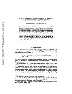
except in the trivial case of constant potential function. It is worth stressing that the operators A and B are the generators of the shifts along the q- and p-axis, respectively. The operators e A~ and e B~, indeed, turn the phase-space vector (q) into (II.3.17)

eA~(:)=(qpPV),

eB~(:)=(p_vq,(q)v),

as depicted in fig. 1. It is needless to say that the mappings (II.3.17) are both symplectic. Then, being the action of the exponential functions of the operators A and B separately known, it is natural to investigate the possibility of expressing the exponential function of the sum as the product of exponential operators e ~AebB with coefficients a and b appropriately chosen. An immediate approach to the posed problem leads to the simple split of the exponential (II.3.13) as the product of the operators (II.3.17), namely [26] (II.3.18)

e(A + B)~ ~_ eA~ eS~ + O ( v 2 ) ,

or, within the spirit of sect. II.2, (II.3.19)

UI(T) = eASe B~,

the subscript stressing that (II.3.19) realizes a first-order integrator. The mapping generated by U1 (T) is obviously symplectic, since it is composed by the two symplectic mappings (II.3.17), i.e. (qn-1, Pn-1)---~(q~, Pn-1) and (qn, p~_l)--~ (qn, Pn) as sketched in fig. 2a).

54


p - V' (q) z eBX

P

iiiiiiii11 eA't

q

q +px

F i g . 1. - Graphic visualization of the shifts acted by the operators e A~: and e 8~ on the phase-space point (q, p).

The differencing scheme generated by Ul(r) is indeed immediately obtained, according to the recipes (II.3.17), in the form (II.3.20)

I qn = qn - 1 + "~Pn 1, -

[ P n = P~- 1 -

"gV' (qn)"

The above scheme exactly conserves the equal-time Poisson brackets {q, p}; we have indeed

(II.3.21)

{ q~, Pn } =

dqn

dpn

dqn _ 1

dq~ _ 1

dqn

dpn

dpn-1

dpn-1

=1,

thus confirming that the first-order integrator U1 realizes a step by step canonical transformation from the initial state to the final state. According to the Zassenhaus formula, that gives the exponential function e (A+ B)~ as infinite product of exponential functions, whose arguments are intrigued expressions involving repeated commutators of A and B, we can write (II.3.22)

e (A + B) -c _~ e A v e B r e -

(v2/2)[A, B] = U1 (T) e - (r2/2)[A, B],

and hence T2

(II.3.23)

IIu(

)- u ( )ll =

-

--~[A,B],

thus confirming that U 1(~') is a first-order integrator, as already pointed out.


55

Finally, let us consider the problem of energy conservation. With the differencing scheme (II.3.20), the Hamiltonian (II.3.11) at t = nr is (II.3.24)

Hn=H(nr)

=

__Pn z 2

+V(qn)=Hn_l

+

rz

--~-p2_lV"(qn_l)+[V'(qn_l)]2}. 2-

"

-

Hence, energy is not conserved by the integrator U1; and the violation is just on the same order of the integrator itself. Furthermore, it is easy to recognize that the term between braces in the above expression results form the action of the commutator [A, B], regarded as the operator (II.3.15) acting on H n - 1 , namely (11.3.25)

Hn =

1 + -~- [A, B]

g n - 1. n-1

Before closing this discussion on first-order sympleetic integrators, let us notice that the simple split of the operator (II.3.17) can be realized reversing the order of multiplication, as well. We can write therefore (II.3.26)

e (A + B) r ~

e B~e AT q_

O(r 2 ),

which gives again a first-order symplectic integrator, let us denote it by uIBA; then, we have (II.3.27)

U1BA(r) = e B~e A~,

where the superscript B A specifies the order of the appareance of the operators A and B in the product. As a consequence, with this notation the operator (II.3.19) should be denoted by uBA(r). The finite-difference scheme generated by (II.3.27) is slightly different from (II.3.19); it consists indeed of two symplectic mappings: (qn- 1, Pn- 1)'--> (qn-1, Pn) and (qn-1, Pn)--> (qn, P~), as shown in fig. 2b). Explicitly, we have (II.3.28)

I q~ = q~- 1 + VPn, [ Pn = Pn- 1 "I;V' ( qn -

a)

-

-

1).

b)

p (qn- 1, Pn)

"~ (qn, Pn)

(qn, Pn)

l

-~ (qn, Pn-1) (qn-l, Pn-1)

q

(qn-1, Pn-1)

q

Fig. 2. - Phase-space picture of the paths, generated by the symplectic splits: (a) u1AB(v) and (b) U18A(r).

56

G. DATTOLI, P. L. OTTAVIANI, A. TORRE a n d L. VAZQUEZ

As before, the ETPB (Equal-Time Poisson Brackets) {qn, Pn } are exactly preserved at each time step, according to that U~A realizes an area-preserving mapping as U~ 8. Finally, the counterparts of the relations (II.3.23) and (II.3.25) are easily written down as 32

IIU(r)- u~A(r)[I = -~-[A, B]

(II.3.29) and 32

(II.3.30)

Hn=H~_l--~{-p2n_lV"(qn_l)+[V'(q~_l)]~}=

{

r2 } 1 - -~- [A, B] n -

H~_ 1. 1

The above relations confirm that the integrators U~r and U~A are totally equivalent as to the basic properties, such as symplecticity and energy conservation. The integration schemes they generate are slightly different, the first approaching the state (q~, p~) anticlockwise, the second, i.e. (II.3.28), clockwise. The accuracy of the schemes is on the first order for both, the only difference being in the sign of the correction to be applied, namely +-(32/2)[A, B], respectively. The choice between the two first-order schemes may be determined by the relative error of the solution, which can be evaluated from the relations (II.3.31)

(qnPn)

= Ul(3)

qn-1 -T-

\Pn-1] -2 \-Pn-l V"(qn-l)

where the signs - and + correspond to the sequence AB and BA, respectively. Different procedures have been suggested to construct higher-order (n 1>2) explicit symplectic integrators for a Hamiltonian of the form (II.2.1). Although ideas underlying the procedures are quite simple, practice is just another thing, the algebra involved in the calculations increasing with increasing the order of accuracy. In the following, we illustrate the differencing schemes generated by the natural generalization of the simple splits U1~B and U~A. In this case, too, the algebra becomes very cumbersome for obtaining integration orders n > 2; alternative methods have been proposed, which practically exploit iteratively the second-order integrator (-72, as it will be illustrated in sect. II.6. II.3.2. Higher-order symplectic integrators. - The visualization of the numerical integration schemes (II.3.20) and (II.3.28) as given in figs. 2 suggests to generate a procedure, which realizes a canonical transformation from the state (qn-1, P n - 1 ) to (qn, Pn) through a certain number of intermediate steps. The symplectic map, which formally represents such zig-zag path is just given by the product of exponential functions of the operators A and B. We write therefore [50-52] k

(11.3.32)

e (A + ~)~ =

[[ ec~A e~J~ + ~(3~+i),

j=l

where the numbers (cj, dj), j = 1, ..., k are to be determined in order to construct an integrator of order n.


57

a)

b) p,

p,

j=k

JskT (qn'Pn)

_[-'-'46 (qn, Pn)

j=k-lT

j =k-1

I

I I

~,j=2

j=2~-"

J=l T

l

A v

J =1

(qn-1, Pn-1)

(qn-l, Pn-1) q

q

Fig. 3. - Phase-space paths, connecting the state (qn-1, Pn I) to the state (qn, Pn) through k consecutive elementary symplectic mappings of the kind (a) (II.3.20) and (b) (II.3.28). The product (II.3.32) stands just as the natural generalization of the simple splits (II.3.19) and (II.3.29), the time steps for each of the mappings, produced by the exponential functions of the generators A and B, are fractionized irregularly into fragments, cjr and djv, of different sizes. It is evident that the operator on the right-hand side of (II.3.32) generates a symplectic flow composed by mappings of the kind (II.3.20), i.e. (II.3.33)

I qj----qj 1-}-cjTpj-1, [ Pj----Pj-1-djTV'(qj),

j=l,

...,k,

which consecutively connect the state (%_ 1, P~-l) to the state (qn, PO, obtained for j = k, as depicted in fig. 3a). It is needless to say that reversing the order of the exponential functions in the product (II.3.32), we obtain k consecutive mappings of the kind (II.3.28), the resulting procedure being visualized in fig. 3b). The direct approach to the problem of finding the set of numbers (cj, dj), j = 1, ..., k, which realize an integrator of the required accuracy, is as follows. We rewrite (II.3.32) in the form k

(II.3.34)

e (A + B)~ = 1-[ ec~A ed'~B f i e ~'R', j= 1

m=2

where the product over m, containing the unknown operators Rm, m 1>2 accounts for the accuracy of the approximation. Then, we take the derivative of both sides with respect to v, multiply on the right by the inverse operator e-(A +B)~ and equate the coefficients of equal powers in v, thus obtaining non-linear algebraic equations for the unknowns (cj, dj) and for the unknown operators Rm, m t> 2.

58

G. DATTOLI, P. L. OTTAVIANI, A. TORRE a n d L. v]tzQut

We report, for instance, the equations obtained from the zeroth, first and secor power in v (see also ref. [44]): k

k

k f

(II.3.35)

j-1

[j-1

]/

q/E ,

k

0, k J- 1 r J 1 j- 1 l Y~ dzldj ~, c~ - - cj ~ di~ j=ll:l [ i=1 2 ,~=1 J

3R~ + 2 ~, [cjA + djB, R2] + [B, [A, B]] • j:l

k [ 1 J J j-1 [j-1 + [A, [A, B]] 2 ] - d j ~, ct ~, c~- cj s c~l Z d t j=l[2

l=l

i=i

/=i

Ll=l

"l'l

dj|[ =, .lj

It is easy to recover the first-order differencing schemes (II.3.20) and (II.3.28) from tk above relations. In fact, with k = 1 we simply obtain (II.3.36)

cl = 1,

dl = 1

from the first of (II.3.35), and hence the second gives (II.3.37)

[A, B] + 2R2 = 0 ,

thus implying (II.3.38)

1 Re = - ~-[A,

B].

The case k = 2 is particularly interesting, since it is possible to generate an explic integrator of the second order, in which one of the exponential functions e A~ or e B~ : symmetrically splitted in two parts. With k = 2 in (II.3.35) we obtain c1+c2=1,

(II.3.39)

dl+d2=l, 2R2 + {cl + c2(d2 - dl)}[A, B] = 0 .

It is possible to choose the parameters (cj, dj), j = 1, 2 to have R2 = 0, i.e. (II.3.40)

cl + c2(d2 - d l ) = 0

or, equivalently, exploiting the first of (II.3.39), (II.3.41)

2 dl (1 - cl) = 2 d l c2 = 1 .

Choosing a symmetric split of one of the exponential operators e A~ or e B~, let us say e A we can put (II.3.42)

1

cl = c~ = - , 2

and hence from (II.3.41) (II.3.43)

dl = 1,

d2 = 0 .


a)

59

b)

p~

9 (qn, Pn)

(qn, Pn)

_7

.t

I

(qn-1, Pn-1)

(qn-1, Pn-1)

q

q

Fig. 4. - Graphic visualization of the canonical transformation produced by the symmetric second-order integrators (a) U A ( r ) and (b) u B ( v ) . The above values of the parameters (cj, dj), j = 1, 2 are compatible with the third relation in (II.3.35), which indeed gives (II.3.44)

1

R3 = ~-~ [A + 2B, [A, B]].

The operator e (A + B)v takes the approximated form (II.3.45)

e (A + B ) r ~_

e

(v/2)A

e vB e (r/2)A + 6 ( 1 . 3 ) ,

where the accuracy of the approximation is on the order: g~(rs). The canonical transformation generated by the map on the r.h.s of (II.3.45) will be more accurately discussed in the next section, and graphically reproduced in fig. 4a). Symmetric split of the exponential operator e ~B is possible, as well. In that case, with d l = de = 1/2, we obtain from (II.3.39) (II.3.46)

C1 ---- 0 ,

cz = 1

and (II.3.47)

1 Ra = - ~ [ B 24

+ 2A,[A, B]].

The operator e (A + B)r is approximated by (I1.3.48)

e (A + B) r ~ e (r/2)B e TAe (r/2)B _{_ ~ ( V 3 ) ,

up to the second order on the time step r, and generates a succession of three symplectic mappings as discussed in the next section and graphically visualized in fig. 4b).

60

G. DATTOLI, P. L. OTTAVIANI, A. TORRE a n d L. V~ZQUEZ

A remarkable features of the integrators (II.3.45) and (II.3.48) is represented by their symmetric structure, which implies the exact time reversibility, expressed in general terms as U(~) U ( - ~) = U ( - T) U(~) = 1.

(II.3.49)

Symplectic integrators with a symmetric form, so that they are exactly time-reversible, are automatically of even order. The integrators on the right-hand sides of (II.3.45) and (II.3.48) have the exact time reversibility (II.3.49) and are of second order. Moreover, the remainder of the difference with the exact operator e (A+B)~ contain only odd powers of v. They are examples of a general statement, which will be demonstrated in sect. II.6, where higher-order integrators (4th, 6th, 8th and so on) are constructed by a symmetric product of symmetric integrators of lower order. In this connection, the symmetric decompositions (II.3.45) and (II.3.48) stand as basic elements for obtaining higher-order integrators. Consequently, we devote wide space to discuss them in some details and illustrate their applications to both classical and quantum mechanics. II.3.3. S y m m e t r i c s e c o n d - o r d e r i n t e g r a t o r s . - Firstly, we consider the symmetric decomposition in (II.3.45), which we denote by UA, where the subscript specifies the order of the approximation and the superscript the operator--A or B - whose action is fractionized into two equal-size steps. Thus [26, 27, 50] U ~ (v) = e (#2)A e ~B e (~/2)A.

(II.3.50)

It is worth stressing that the above integrator can be understood as composed by the product of two simple splits of the type discussed in sect. II.3.1, corresponding to the half-time increment v / 2 , namely (II.3.51)

:

which generates two subsequent mappings: from (qn - 1, Pn - 1 ) to the intermediate state (qn-1/2, Pn-U2), obtained from the scheme (II.3.20) for a half-integral time-step v / 2 and then from (qn-1/2, Pn-1/2) to the final state (qn, Pn) through the scheme (II.3.28), applied for a time shift v/2. The path of fig. 4a), indeed, can be regarded as resulting from the sequence of the paths of fig. 2a) and 2b). With the explicit form of the operators A and B, given in (II.3.14), we obtain the second-order symplectic integrator U2A (T) = e (v/2)pgqe - ~v' (q)ape (v/2)pgq,

(11.3.52)

which generates the explicit differencing scheme 2

qn-1 + -~Pn-1

(II.a.53) Pn

= Pn-

1 -- v V '

q~- , +

Pn- 1 9

~qn-1 + ~(Pn-l§


61

Because it is composed by symplectic mappings, the integration scheme (II.3.53) is symplectic. In fact, it is easy to verify that the ETPB is preserved, being exactly (II.3.54)

{qn, Pn} = 1

if {qo, Po} = 1.

On the other hand, the Posson brackets at different times are q.} = 3 (II.3.55)

{Pn-l, P n } = v V " ( q n - l + 2Pn-1 ), as a consequence of the discretization. According to the results of sect. II.3.2, we can write (II.3.56)

lie _ :H:~_ U~(v)II..~ -r~~[ A + 2 B , [ A ,

B]] = --:33 24 _ p 2 V , , + 2 V , 2 : .

As for the energy conservation, with the explicit expressions (II.3.53), we find (II.3.57)

H n --

__P2 2

T3

+ Y(qn) = H n _ l + =--:{p3_lIY"(qn_ 1) -- 6pn_lV'(qn_l)V"(qn_l)}. 24-

As already remarked, energy is not conserved; the correction at each step is just on the same order as the integrator itself. Furthermore, on account of (II.3.56), one obtains T3

(II.3.58)

H n = H ~ - I + - - : - p 2 V " + 2V'2: Hn-1. 24

1'he violation to Hamiltonian invariance: Hn ;~ Hn 1 is quantified by the remainder in (II.3.56), where the partner in Poisson bracket is provided by Hn-1, i.e. the Hamiltonian at the preceding time step. The transformation from the initial (qo, Po) to the final state (qN, PN) is obtained by applying N times the integrator (II.3.52). In symbols,

and, since the error cumulates at each step, the accuracy reduces to N r 3 = Tv 2. This can limit the application of the numerical integration scheme (II.3.53) in eases where many time steps are required, as for instance in the treatment of charged beam transport in circular machines. We consider in detail the operator in (II.3.59). Multiplying m integrators of the kind (II.3.52), we formally find (II.3.60)

[uA(v)]m=U~ AB -~ [ u A ( v ) ] m - I u

~

,

m~>l,

62


a)

b)

U AB ('c/2) (qN, PN)

O-/"T (qN, PN) __J

U~ A (~/2)

-~ f-.-

!

(_

I

~ - ~ U BA ('c/2) (qo, Po) 1

N-1

(qo, Po) I,.

q

ID

q

Fig. 5. - Phase-space paths generated by the symmetric integrators (a) uA(v) and (b) UB(v), connecting the initial state (q0, P0) to the final state (qN, PN) through N consecutive v-steps.

which displays an interesting symmetry. The structure of the above operator reproduces indeed that of the integrators U2(v) themselves, thus providing a useful scheme from a numerical point of view. It is apparent thereby that m consecutive applications of U~(v) are equivalent to the following sequence of maps: - first-order integrator -

U BA (v/2),

second-order integrator resulting from the previous step: [UA(v)]m- 1,

- first-order integrator

uiAB(v/2),

which generates the path in phase-space sketched in fig. 5a). We consider now the product on the right-hand side of (II.3.48), in which the exponential functions of the operator B, i.e. e (ff2)B, are symmetrically placed with respect to e ~A. According to the adopted notation, we can write therefore (II.3.61)

U B (3) = e (~/2)8e ~Ae (v/2)B.

It is immediate to recognize UB(r) as generated by the product of two first-order integrators as in (II.3.51) although in the reverse order, namely (II.3.62) According to the phase-space path of fig. 4b), it produces two mappings having the point (qn-1/2, Pn-1/2) as intermediate state, as (II.3.51), the sequence of the two paths being obviously inverted.


63

Specifying the form of the operators A and B as in (II.3.14), we obtain for the Hamiltonian (II.3.11) the further second-order symmetric integrator

UB ( v ) = e-(~/2)V'(q)aPe~Paqe-(z/2)V'(q)ap,

(II.3.63)

which generates the integration scheme

{ qn = qn-1 + "~Pn-1 -- V 2 V ' ( q n - 1 ) , 2

(II.3.64)

T pn=Pn-i - -~[V'(qn-i)+

V'(qn)],

corresponding to the phase-space path of fig. 4b). Symplecticity is obviously preserved by the scheme (II.3.64):

{ qn, Pn } = 1,

(II.3.65)

although the discretization affects the different time Poisson brackets, being

{Pn-1, Pn} = -~V (qn-1) 1 + 1 - -~

(II.3.66)

V"(qn) .

Finally, using (II.3.47), we can write (II.3.67)

lie -:H:~

uB(v)]I =

1-3

T3

Z4

24

~--:[B+2A,[A,B]]

2p2V" + 2V'2:.

It is worth stressing that the difference evolution equations (II.3.64) can be derived from the so-called leap-frog scheme, defined by

I qn+l = qn + VPn+(1/2), (II.3.68)

[ Pn+ (1/2)

=

Pn -

(1/2) --

TV' (qn),

where the auxiliary momemta Pn- 1/2 and Pn + 1/2 must be understood as corresponding to half-integral time-steps. As noticed in ref. [24], we can define the momenta Pn, relevant to integral time steps, as the averages 1

Pn = -z (Pn +1/2 -~- Pn - 1/2)

(II.3.69)

Z

which, once combined with (II.3.68), yield the scheme (II.3.64). As before, the symplectic symmetric integrator (II.3.63) does not conserve the energy; with the evolution specified by (II.3.64), it is easy to obtain 7y3

(II.3.70)

Hn = H n _ l + --:-:~{ p 3 _ l V " ( q n _ l ) - 6Pn_l V ' ( q n _ l ) V " ( q n _ l ) } , IZ

64


which can be rewritten as 753

(II.3.71)

Hn = H~_ 1 - - - : - 2 p 2 V " + V ' 2 : 24

H~_I,

thus confirming the crucial role of the remainder in (II.3.67) on quantifying the violation of energy invariance. We briefly comment on the iterative process leading to the final state. In formal terms, the state (qY, PN) at time T = NT is obtained from the initial state (qo, Po) at time to -- 0 by means of the product of integrators: =

pN

2

2

p0"

As depicted in fig. 5b), it is possible to recognize in (11.3.72) a sequence of integrators, similar to that generated by (II.3.60). In the above expression, the first-order integrators contribute to the sequence in the reverse order with respect to (II.3.60) and, furthermore, the nucleus of the procedure is given by the second-order integrator [U2B(T)]N - 1 resulting from the previous step. As final comment, we notice that the schemes (II.3.53) and (II.3.64), generated by the two second-order symmetric integrators (II.3.52) and (II.3.63), respectively, are not fully equivalent. Choice between them should be made according to (II.3.57) and (II.3.71), which specify the deviations from the energy conservation. In this connection, we point out that the error on the solution (qn, Pn) of the equations of motion can be evaluated according to the relations

11) / .g3

(II.3.73)

T3R3(~

-1 V (qn- 1)

~ -~\4VP(qn_i)Vr(qn_i)_p:

1Vm(qn-1)

)

for the scheme (II.3.53), and (II.3.74)

va R3 qn-1 = Ta 2 " \Pn-1] - --~ V ' ( q , ~ _ 1) V"(qn-1) - pn2- 1 Vm( -(tn- 1)

for the scheme (II.3.64). Before closing this section, we stress that the difference evolution equations (II.3.53) can be derived from a scheme similar to the leap-frog scheme, with the role of the coordinates p and q being interchanged. Introducing auxiliary coordinates, qn-1/e and qn +1/2, defined at half-integral time-steps, we consider the equations [24] (II.3.75)

I q'~ § 1/2 = q n - 1/2 + rpn ,

[ P~ + 1 ~-- P~ -

r V ' (qn + 1/2 )"

Then, defining the coordinates qn in similar fashion as in (II.3.69), i.e. (II.3.76) we obtain the scheme (II.3.53).

1 q~ = -~ ( q ~ - 1/2 + q~ + i/z) ,


65

II.4. - L i o u v i l l e e q u a t i o n and d i f f e r e n c i n g s c h e m e s

In the previous sections we have investigated the possibility of developing numerical integration methods to solve the problem of the motion of a classical system under the Hamiltonian H(q, p) = T(p) + V(q). The problem has been posed within the context of the Hamilton equations of motion for the canonically conjugate variables q and p. Symplectic integrators of first and second order have been constructed to generate explicit differencing schemes, which provide approximated solutions to the equations of motion in form of a grid of values (qn, Pn) at discrete time-steps tn = nv, n = 0 , 1, ..., N. As is well known, the Liouville equation represents an alternative tool to describe the evolution of a classical system with respect to the Hamilton equations of motion. Let be Q(q, p, t) the phase-space distribution function, where, as in sect. II.2, q and p are allowed to denote the n-component vectors (II.2.2). The evolution of Q(q, p, t) under the Hamiltonian H occurs according to the Liouville equation, which writes (II.4.1)

3 -:-: Q(q, p, t) = {H, Q}.

d$

With the notation of sect. II.3, eq. (II.4.1) can be recast in terms of the Lie operator :H: as

9 3t ~) = : H: Q,

(II.4.2)

thus more clearly displaying its operatorial nature. It is worth noticing that the notation adopted in sect. II. 3, reproduced from refs. [19, 28], is usually limited within the context of Hamilton picture. We prefer to extend it to the Liouville equation as well, in order to avoid proliferation of notations and to evidentiate the analogy between the two approaches to the classical problem of the dynamics of a Hamiltonian system. The formal solution to eq. (II.4.2) is given as (II.4.3)

Q(q, p, t)

=

e:H:(t-t~

P0, to),

where P(q0, P0, to) - r represents the distribution at the initial time to and the o p e r a t o r e :H:(t-t~ turns the distribution function at to into the distribution function ~)(q, p, t) at time t. According to the Liouville theorem, the operator e: H: t is symplectic. The question is therefore the same as in sect. II.2: if the time-step v - t - to is assumed small, is it possible to find an approximate form of the evolution operator U(T) - e: H: 9 up to a given order of accuracy? In this case, indeed, iterating the process we can determine the distribution function r as a grid of values {~)~} at the discrete times t~ = nT. Denoting by Urn(T) the m-th order integrator, as in sect. II.2-II.3, we can formally write (II.4.4)

~ n ~- ~(tn) : [Vra(T)]n ~o,

which, once the explicit form of Urn(T) is given, provide the differencing scheme to solve the Liouville equation (II.4.1).

G. DATTOLI, P. L. OTTAVIANI, A. TORRE and L. V~,ZQUEZ

66

It is immediately recognized that the evolution operator relevant to eq. (II.4.1), /~e. (II.4.5)

U(v) = e: H: r,

reproduces just the operator in (II.3.7) relevant to the Hamilton equations, if the time step r is replaced by - v . This is a general statement regarding the relation between the symplectic map Un, generated by the Hamilton equations of motion, and the symplectic operator UL, associated to the Liouville equation: (11.4.6)

U L ( t ) ---- y i ~ l ( t )

-- U H ( - t ) ,

where the subscripts L and H stand for L i o u v i U e and H a m i l t o n , respectively. We add them to the symbol U to precise the context we are working in. In this section we omit to sign the subscript L, since the discussion concerns exclusively the Liouville equation. All the results of the previous sections as to the symplectic integrators hold unchanged [26, 27]; we simply need to replace r with - r. In addition, let us notice that according to the Liouville theorem the effect of the operator U ( v ) = e :H: 3 on the distribution function Qo at time to can be reported on the variables q and p as (II.4.7)

e:H: 3r

Po) = ~)o[q(r), p(r)],

where the new arguments q and p of ~)0 are just obtained from (qo, P0) through the operator e :H: 3, namely (II.4.8)

q(r) l = e:g:3(qoPo).

As a consequence, eq. (II.4.4) generates, in correspondence to specific forms of the m-th order integrator U,,(r), differencing schemes for the variables (q, p) regarded now as arguments of the distribution function •, rather than as vectors in the phase space ~2n. We can reproduce all the schemes, obtained in the previous section, with the substitution r - * - v . We report them below in table form. Considering the Hamiltonian of a single particle acted by the potential V(q): p2

H = -2

+ V(q),

we get: - First-order integrators The first-order integrator (II.4.9)

U1A~(r) = e -p3aqe 3y'(q)ap

generates the finite-difference scheme: (II.4.10)

I q~ =

{ Pn

q n - 1 -- T P n - 1,

= Pn-1

+ vV'(qn).


The error is as before given by 1.2

IIuH. III.3. - Spectral estimations in the Heisenberg picture

The finite-difference schemes to solve the Heisenberg equations can be used to obtain estimations of the energy spectrum [60,63,29,68,72]. The method in the Heisenberg picture is based on a variational approach to the matrix elements: (III.3.1) (III.3.2)

( E m l O ( t ) IEn) = e~-~(E~-Em)t~(Em ] 0 ( 0 ) j E n ) =

= (Era I O ( 0 ) I E n ) E [ - i ( E n - E r a ) t]k k k! '

where I E n ) and IEm) are eigenvectors of the Hamiltonian H, and O(t) is any operator associated to the quantum system. Any discretization of the Heisenberg equations defines an approximation to eq. (III.3.2). On the other hand, we have to consider a suitable approximation to the eigenstates IEn). From this approximation and by consistency arguments we obtain estimations of the energy levels [72] and the energy differences independently [60, 63, 29, 68]. The accuracy of the method is related to the accuracy of the Heisenberg finite-difference scheme as well as the accuracy of the approximated eigenstates. To illustrate the method we will consider three applications in the next subsections. III.3.1. O n e - d i m e n s i o n a l q u a n t u m systems. - To illustrate the two possible spectrum estimations, let us consider the one-dimensional quantum system: (III.3.3)

1 H = _ p2 + V(q). 2

- C o m p u t a t i o n of the energy levels [72].

In this case, we consider the matrix element between the same eigenstate which


109

using (III.3.2) yields (III.3.4)

,

which is the expression of the virial theorem and it turns out to be the minimization condition in ~ of the matrix element (En [HIEn) with (III.3.10)

IE~} -'-->~/) n

: V~)(~/X) 9

That allows us to estimate the energy levels of H in terms of the variational parameter. The accuracy will be related to the accuracy of the variational states IEn). As a consequence, we have a justification of the variational method of Dias de Deus et al. [78-80] in the context of the Heisenberg picture. On the other hand it represents a generalization of the method of refs. [60, 29, 68] which only allows us to compute the energy differences. In table I, we show the estimated values of the energy levels for the quartic anharmonic oscillator, and compared with the exact results. The states of the harmonic oscillator are used as variational states IE~).

- Computation of the energy differences [60, 63, 29, 68]. By using the same unitary difference scheme as before and considering the operators q(t) and p(t), we obtain (111.3.11)

(Era Iq(T) ]En) = (Em]q(O) IEn} + 3(Em Ip(O) IEn)

(III.3.12)

(Era Ip(3) ISn} = (E,~ Ip( O) [Sn} + 3(Era IF(q( O) ) ISn) + 0(32).

+

0(32),

110

G. DATTOLI,P. L. OTTAVIANI,A. TORREand L. V~ZQUEZ

TABLE I . - E s t i m a t i o n of the energy levels of the quartic anharmonic oscillator 2q4 in units

~1~.

State no.

Exact results

Estimated energies

0 1 2 3 4 5

0.6680 2.3936 4.6968 7.3367 10.244 13.379

0.6814 2.4237 4.6850 7.2911 10.167 13.267

TABLE II. - Estimation of the adjacent energy differences

0 n = En+ 1 -E

n of

the quartic

anhavmonic oscillator ~q 4 in units ~ 1/a. O n

Exact results

Energy differences from the estimated levels

Energy differences obtained directly

o0 01 02 w3 04

1.7256 2.3032 2.6399 2.9073 3.1350

1.7423 2.2448 2.6061 2.8759 3.1000

1.8171 2.2894 2.6207 2.8845 3.1072

By imposing the consistency of (III.3.2) and (III.3.12) up to the first oder in ~ we obtain (III.3.13)

1 (Emlp(O)IEn)

w= -

i (E,~lq(O)[En) '

(III.3.14)

w-

1 (Era [F(q(O))IEn} i

,

(Emlp(O) lEn}

where w = E ~ - E n. In order to satisfy this we introduce the same variational parameters as in (III.3.7). Thus we obtain (III.3.15)

(E IplEn} _ 7a (E lF(Tx) IEn) (EmlxlEn) (EmlPlEn)

As an illustration and, as before, for the quartic anharmonic oscillator, we show the adjacent energy differences in table II. III.3.2. Two-dimensional q u a n t u m systems. - In this section we consider a general quantum system with two degrees of freedom in the Heisenberg picture. By using an explicit unitary discretization we obtain partial information about the energy spectrum of the generalized quantum Henon-Heiles system [68].


111

Let us consider the quantum system 1

H = _ ( p 2 + p2) + V(q, Q). 2

(III.3.16)

The Heisenberg equations of motion are the following: dq

(III.3.17)

dt

dQ

(III.3.18)

dt

dp

- p ,

dP

- P,

3V

-

dt

aq

3V

-

dt

3Q

and q(t), p(t), Q(t) and P(t) are operators which must satisfy the equal-time commutation relations [q(t), p(t)] = i ,

(III.3.19)

[Q(t), P(t)] = i .

The quantum-mechanical problem consists of solving the ordinary differential equations (III.3.18) for the operators q(t), p(t), Q(t) and P(t) with the constraints (III.3.19). A consistent unitary discretization of (III.3.18) is the following explicit scheme: (III.3.20)

(III.3.21)

qn+l -- q~ r

Qn+l-Qn r

Pn+l -- Pn

- Pn + 1,

r

--

Pn+l--Pn

- P~ + 1,

v

aV(q~, Qn)

-

aq

,

9V(qn,Qn) aQ

,

where qn, Pn, Qn, Pn are the operators q, p, Q, P at time t = nv. It is easy to verify that the scheme preserves the equal-time commutation relations (III.3.19) and it is a generalization of the scheme (III.2.19) for one degree of freedom. The simplest way to obtain information about the energy eigenvalues is to study the time dependence of the operators q(t), p(t), Q(t), P(t) for short times (one time step with the help of a unitary scheme). To this purpose, we introduce the set of Fock states In, N> generated by the operators a, a t, A, A , defined in terms of qo, Po, Qo, P0 as follows:

(III.3.22)

a(a + a t) qoV~ ,

(a-a t ) p o - iaV~ '

fi(A + A t) (III.3.23)

Q0 -

(A - A t) ,

P0 -

,

where a and fi are variational parameters to be fLxed by a simple self-consistency requirement. The operators a and A satisfy the commutation relations (III.3.24)

[a, a t ] = i ,

[A, A t] = i .

112

G. DATTOLI, P. L. OTTAVIANI, A. TORRE and L. VJ~ZQUEZ

According to eqs. (III.3.18) we take the matrix elements (III.3.25)

(z[ql lY;>, (ZIP1[F>,

(III.3.26)

,

0 there are either two or no roots according to the values of n and N. This result has been checked numerically for different cases. In table III, the numerical results for two representative examples are shown. The results indicate that the structure of the discrete spectrum, obtained in the framework of the above approximation, depends only on the sign of ~t. On the other hand, the classical integrability of the system depends on the sign of )[ and the values of the frequancies A and B. This result fits with the results of Casati et al. [83], in the sense that the classical phenomenology of the system is richer than the quantum one. III.3.3. The hydrogen atom in a magnetic field. - In this section we show other spectral applications of the unitary time discretization of the Heisenberg equations [69]: an approximate nonperturbative expression is obtained for the level splitting in the Lz = 0 sector of the hydrogen atom in a magnetic field. The hydrogen atom in a magnetic field is of special interest because it is a quantized version of a nonintegrable system which is accessible to experiments [84-86]. As in the previous applications, the analytical estimate of the level spacing is obtained by matching the short time evolution of distinct operators and using an adjustable parameter which perform a scale transformation for each vector in a basis of eigenstates of the integrable system. In this way, we obtain a result that extrapolates beyond the perturbative results in the low magnetic-field limit. The Hamiltonian for one electron in a Coulomb potential and a magnetic field B along the z-axis is (III.3.39)

p2 H . . . . 2

1

y y2 + -- (L~ + 2Sz) + (x 2 + y2) r 2 -8-

in atomic units, with ~ = B(4zeo)2h3/(m2e~). We will study the Lz = 0 sector in the situation where the quadratic Zeeman term dominates the spin effects. Then the Hamiltonian becomes p2 H . . . . 2

(III.3.40)

1

~2 + __ (x 2 + y2). r 8

Thus, we have the eigenvalue problem H T = EW. With the semiparabolic change of coordinates (III.3.41)

q -- ( -2E)l/4(r + z) ~/2,

Q = ( - 2 E ) l / 4 ( r - z)1/2

we obtain 5~ = 2 e ~, where (III.3.42) t ~ V = - - l ( - - a 2 + - 1 ) 9_ _ 2 aq 2 q 9q

lq2 - 1 (~ 1 9) 1 2 ~'22 2 +Q2), 9 -~+-Q 3-Q + - 2 Q + 8 q Q (q


115

where (III.3.43)

s = 1/( - 2E) 1/2,

(III.3.44)

~ = ~ / ( - 2E) 2.

In our analysis we will consider the levels of the (equivalent oscillator) problem defined by the Hamiltonian t ~ . The levels of the original hydrogen atom problem may then be obtained from eq. (III.3.43). The new coordinates q and Q may be interpreted as radial components of two bidimensional harmonic oscillators. Thus we obtain

(III.3.45)

~ -

2 1 ~_~(p~+q~)+ 1 E2 ( P ~ + Q ~ ) + - ~~q 2-~2( ~ q 2 +Q2), -2 i= 1

2 i= 1

where q = (q~ + q~)1/2 and Q = (Q~ + Q~)I/2, being qi and Qi Cartesian coordinates in R 2"

Following the same steps than in the previous section: the time discretization of the Heisenberg equations and the introduction of the Fock spaces In, N} with variational parameters. These states are not eigenstates of the Hamiltonian ~ but they are actually supposed to provide a set of labels for the states of the perturbed problem. We obtain analogous equations to (III.3.36)-(III.3.38), and from them we obtain the energy difference (III.3.46)

w 2 = 2 + ~/4 + 2)~(g(N) + 4tth(n, N ) ) ,

where g ( N ) = 3 ( N + I ) 2 + 3 N 2 + ( 2 N + 1 ) 2, h ( n , N ) = ( 2 N + l ) ( n + l ) and ~ = 2 . 5 being the best estimate obtained by matching the short-time evolution of the Heisenberg operators and the standard perturbation results [68]. From (III.3A6) we obtain: 1) Conditions for the overlap of the diamagnetic multiplets are established for states near the ionization threshold; 2) the clustering of levels at the upper side of diamagnetic multiplets is also observed.

III.4. - The quantum field t h e o r y on a Minkowski lattice A quantum field equation is simply a partial differential equation of operators. In the case of nonlinear quantum fields we have three methods of study: 1) Rigorous mathematical approach. This line of work has been developed, mainly, by the school created by J. Glimm and A. Jaffee [87]. 2) Numerical approach. This method allows us to make nonperturbative computations in quantum field theory and it is based on the numerical estimation of functional integrals using a Monte Carlo algorithm. The different aspects of this method are described by Creutz [88]. 3) Minkowski lattice approach. This method consists in the application of the finite-difference method to solve the partial difference equations of operators which appear in quantum field theory. This method had been developed by Bender et al. [23, 63] and V~zquez [29, 66].


116

III.5. - The n o n l i n e a r K l e i n - G o r d o n q u a n t u m field t h e o r y

Let us consider the quantum nonlinear scalar field theory in (1 + 1 ) dimensions (III.5.1)

q~ tt - q~ ~ + f(q~) = O .

Let us rewrite the operator field equation as follows: (III.5.2)

//t = ~xx - - f ( ~ ) .

~t =//,

We have to solve the system of partial differential equations in operators (5.2) subject to the constraints (III.5.3)

[q~(x, t), I I ( y , t)] -- i S ( x - y ) ,

(III.5.4)

[q~(x, t), q~(y, t)] = O,

(III.5.5)

[ I I ( x , t), I I ( y , t)] = O.

Let us consider the following two unitary (III.5.2)-(III.5.5): - Explicit

(III.5.6)

s c h e m e [66,29]

r

1- ~ T

(III.5.7)

schemes associated to the system

///n + 1 - - / 7 / v

-- / - / nt + l ,

-

~ l n + l - 2~tn + ~bln- 1 h2

_f(r

where ~ = q~(nT, lh). The scheme is local: the value of the field q~+l depends on the values of the field at the time levels n and n - 1, and it preserves the equal-time commutation relations: (111.5.8)

[r

= /h5 lk,

(II1.5.9)

[q~, r

= 0,

(III.5.1O)

[H~, Hkn] = 0.

- Implicit

(111.5.11)

(III.5.12)

(111.5.13)

(III.5.14)

s c h e m e [23, 63]

~/}1n + 1 q- ~/n+ll -- ~/n -- ~/n -1

2v r

=

/-/n1 + 1 + /-//n-+ll + /-//n + ///n- 1

4 +

~ n[-1 + l q_ ~/n-- ~/n -1

2h

+1, +

+

-1

4

i / nl+ 1 + /-//n-+ll _ 117/ _ /--//-1

~//n +1 -- ~[//n+11 q- ~tr'//n-- ~r-//n- 1

2~

2h

-f

[1

]

-~ (~/)/n+l "~- ~/)/n+11 "~- (/}/n q- ~/)/-1) .

117


The scheme preserves the equal-time commutation relations (III.5.10) but it is not local and involves a great algebraic complexity. The results obtained on the lattice are consistent with those known for the underlying continuous system. In the next sections, we present some spectral estimations obtained with the explicit scheme and by considering the nonlinear term as the normal product : f(q~):.

III.5.1. The ~4 quantum field theory. - Let us consider the real scalar quantum field theory [66, 23, 63]: (III.5.15)

~)tt - -

m 2 r + ;~q)3 = O .

~) x x +

In order to obtain basic spectral estimations, let us consider a generalization of the method used for the one-dimensional quantum oscillator in the context of the above explicit scheme. Let us consider one time step iteration and compare the operators q~Zo,//to and q~~, H~, by assuming periodic boundary conditions such that 0 ~ 0 and 2 R > 0 we can easily see that there is only one solution of this kind. Since t~l > ~90 = m, no spectrum exists in the interval (0, 2Q0) which should correspond to the absence of two-particle bound states of the single phase of the 0 4 model [87] we have considered. - If ;t < 0, the theory is not totally established (the Hamiltonian is not bounded below). In the framework of the present approximation we obtain the existence of a

EVOLUTION OPERATOR EQUATIONS: INTEGRATION WITH ALGEBRAIC ETC,

119

finite number of bound states, being the number fLxed by the condition 2m 2 I)~R In ~< - -

(III.5.29)

Remark. (III.5.30)

If we consider the general nonlinear quantum Klein-Gordon model ~) tt - - ~) xx + m 2 r + ~ 2 N -

1 = O.

And the spectral estimations are made with the implicit scheme (III.5.14) and without the normal product of operators, we obtain the renormalized mass (III.5.31)

m~=m2+

(2~)y_ I

In ~

It is almost identical with the ordinary perturbative renormalization formula. III.5.2. The sine-Gordon q u a n t u m field theory. - Now, we have the real scalar quantum field theory [63, 29]: (III.5.32)

m3

~9 tt -- ~) xx "F

V~

---~ sin --m r 1 632= 0 .

Proceeding with the explicit scheme as in the previous section for the q~4 model, we get the following equation for the separation of the levels of the mass spectrum: (III.5.33)

~n $9n+2 = m2n! ~_~ ;LkR$gVn-k

k =0

1

k!(k + 1 ) ! (n - k) !

being $9n = E n + l - E n , and the renormalized coupling constant is introduced as follows: ,~/(2Lm 2) ---->,~R. The following features of the spectrum arise: - F o r n = 0, we have $9 0 = m so there is no mass renormalization. If )l = 0, we get $9n = m, as it is expected for the free massive Klein-Gordon quantum field. - F o r each n there is only one positive root of (III.5.33), and $9 n

+

1 > $9 n "

- There is a countable number of particle states in the spectrum of the quantum sine-Gordon field. By an appropriate choice of the coupling constant )[ R some of these states can be identified with the doublet states obtained by Dashen et al. [89]. The other states would define quantum multisoliton states. F o r instance, let us identify E1 = m + $9 1 as the quantum soliton (antisoliton) state. Then the state E2 = m + $9 1 + $92 can be identified with a doublet state provided $92 < m + $91. This condition imposes a bound on the coupling constant ;t R, similar to the one obtained in [89].

Remark. By using the implicit scheme [63] the following nonperturbative result is obtained for the mass renormalization: 2)l(S~-~'l m~)

(III.5.34)

m R =m

(am)(~lm T

120

G. DATTOLI, P. L. OTTAVIANI, A. TORRE and L. V~.ZQUEZ

III.6. - Open questions

As in the case of the Heisenberg equations of a particle, the following open questions appear about the finite-difference equations of operators obtained from the quantum field equations: 1) The study of the relation between the results on the Minkowski lattice and the properties of the underlying continuous system. 2) Convergence of the theory based on the lattice when h, T--) 0. 3) Stability of the finite-difference approximations. 4) The study of the relation between the theory of the classical finite-difference equations and the theory of the quantum finite-difference equations. In this monography, we did not discuss the linear SchrSdinger field on a Galileo lattice [48] and the linear Dirac field on a Minkowski lattice [23, 49, 90]. In both cases the main effort has been devoted to define a physically consistent discretization on the lattice. In the case of the linear Dirac field, the physical conditions to be satisfied are the following: (1) the action must be Hermitian, (2) the fermion doubling must be eliminated, (3) chiral invariance should occur in the massless theory, and (4) the equal-time anticommutation relations must be preserved. In the above references such properties are discussed in terms of explicit and implicit schemes.

During the completion of the paper the authors have benefitted from discussions with various collegues. In particular they express their sincere appreciation for the kind interest and encouragment of Prof. W. WITSCHEL,Dr. M. QUATTROMINIand Mr. G. MAZZACURATI.This work has been partially supported by the Human Capital Mobility Program (Network CT94-0480). One of the authors (LV) acknowledges the support from the Comision Interministerial de Ciencia y Tecnologia of Spain (grant PB95-0426).

APPENDIX A

Generalized forms of Hermite polynomials generating functions

In the ftrst part of this review paper we have analyzed the importance of the Hennite polynomials and of their generalized forms in the framework of operational calculus: we have seen that the theory of generating functions plays, within this context, a not secondary role. Their direct use is not infrequent in the treatment of physical problems like those related to the theory of squeezed states. Generating functions of the type zjn +k

(A.i)

~ ( j , k; z, x, y) = ~, Hjn+k(x, y) n=o (jn + k)!

for arbitrary integers j/> 1 and k t> 0, have been discussed in refs. [91].


121

To obtain an explicit expression for eq. (A.1), we first state the value of zJn +k

(A.2)

J(j,

k; z, x, y) =

By keeping k = 0, we note that J

n=o ( j n + k)!

satisfies the differential equation aJ

(A.3a)

-- J 3z j

= J

with the complementary conditions (A.3b)

J]z=O = 1

-'

It is clear that J

J

= 5z, j,

3Z ~

fl < j .

z = o

must be of the type J

(A.4)

J

= ~ a,~exp [ze 2~i(m/j)] 7~= 1

with the coefficients a m defined by the relation J

(A.5)

~ a m e ~im(~/j)= 5j,~, m=l

which is easily shown to be satisfied by (A.6)

1

a ,~ -

J The extension to the case k * 0 derivative

is obtained by using the notion of negative T

1

(A.7)

b ~(n

f(v)

-

f

(n - 1)!

(r - ~)~- 1 f ( ~ ) d ~ .

b

The previous relations yield (A.Sa)

J(j,

z

if

0; z) - ( j - 1)!

(z

-- ~ ) j - 1

•(j,

0; ~) d~

o

and thus z

(A.8b)

J(j,

k; z) = ( j + k - 1)!

(z

-- ~ ) j + k - 1

j(j,

o

which yields (A.9)

J(j,

k; z) =

1 3 /=1

e x p [ ze 2~i(m/J ) ] e 2~i(m/j)

0; ~) d~,


122

We can now derive (A.1) in a fairly straightforward way, we set indeed (A.10)

~ ( j , k; z, x, y) = e y(~/a~2) ~ (xz)jn+k n=0 ( j n + k)!

= ey(~/ax~) _1 ~ exp[zxe 2=i('~/j)] = _1 ~ j ~=1

j

(e2ni(m/J)) k

m=l

exp[z2ye4~(m/i)]exp[zxe 2~i(m/j)] (e2~i(m/J)) k

The extension to polynomials H(nm)(x, y) is also easily obtained, in fact (A.11)

$'(~)(j, k; z, x, y) =

1

e x p [ z m y e 2mzi(h/J ) ] e x p [zxe2~i(h/J ) ]

~_~

(e2~i(h/J)) k

J h:l

A final important example is provided by the sum zjn +k

(A.12)

t~V(j, k, p, q; z, x, y) ---Hjn+k(X, Y). n=o (pn + q)!

Accordingly, we note P exp[zJ/Pe 2~i(h/p)]

Z jn+k

(A.13)

J(j,

k, p, q; z) =

--zk-(Jq/P) Z h=1 n =0 (pn + q) !

(e 2hi(h/p) )q

Therefore, by applying the same method as before we find (A.14)

:~V(j, k, p, q; z, x, y) = e y(~/ax2) • ( j ,

4~f~_ The above integral representation whenever

kp, q; zx) =

exp

can be reduced to simple Gaussian forms

in k - "---~ -positive integer, P

(A.15)

~-y

i ~ ~

Evolution operator equations: Integration with

Evolution operator equations: Integration with

Suggest Documents

Elliptic Quadratic Operator Equations

Numerical integration of stochastic differential equations with ...

Abstract Semilinear Evolution Equations with Convex-Power

INTEGRABLE EVOLUTION EQUATIONS WITH CONSTANT SEPARANT

Functional Evolution Equations with Inﬁnite Delay

Solving differential equations with grammatical evolution

Exact treatment of operator difference equations with nonconstant ...

Sparse finite element methods for operator equations with stochastic ...

Differential Operator Equations with Interface Conditions in Modified

Linear operator equations with applications in control and signal ... - RPI

Rough evolution equations - arXiv

Fixed Point Theorems on Nonlinear Binary Operator Equations with

Classifying evolution equations.

Adaptive wavelet methods for solving operator equations

Stochastic Integration of Operator-Valued Functions with Respect to ...

sectorial evolution equations - Semantic Scholar

nonlinear evolution equations - Project Euclid

Thermodynamic hierarchies of evolution equations

Integration by parts formula and applications to equations with jumps

Integration of Langevin Equations with Multiplicative Noise and ...

Evolution equations associated with the subdifferentials - Project Euclid

Stochastic Evolution Equations with Multiplicative Poisson Noise and ...

A new approach to stochastic evolution equations with adapted drift

Existence of solutions for impulsive fractional evolution equations with