Linear operator equations with applications in control and signal ... - RPI

LECTURE NOTES

Linear Operator Equations with Applications in Control and Signal Processing

T

he development of mathematical systems theory is arguably one of the greatest achievements of the 20th century [1]. A few key concepts have enabled this development, one of which is linear operator equations. Problems that give rise to linear operator equations include linear regression, optimal resource allocation, optimal filtering, optimal control, and solutions to integral and partial differential equations, to name but a few. Given the wide variety of problems that can be posed as linear operator equations, an ability to pose and solve them is one of the most important tools that systems engineers can have in their “bag of tricks.” The objective of this article is to present the essential ideas behind the solution to linear operator equations. The intended audience is graduate students specializing in control and signal processing. Although linear operator equations are presented and studied in numerous textbooks, they are usually studied in the context of specific applications. Here we present a unified framework for linear operator equations in a way that we hope is insightful. In addition, we offer several common examples to illustrate some potential applications. We will study equations of the form A x = b, where A is a linear operator and b is given. The objective is to find an x that satisfies the equation. The theory discussed in this note is subject to the following assumptions: • The operator is linear and maps one Hilbert space to another Hilbert space. This assumption limits the scope of application to spaces with a well-defined inner product, which excludes, for example, the space of bounded signals (L∞ ). • The operator must be bounded. This assumption limits the scope of application to continuous operators, which excludes, for example, partial differential equations. • The range space of the operator must be closed. This is a mild assumption that is satisfied by almost all interesting bounded linear operators from one Hilbert space to another. Although these three assumptions may appear limiting, they include a large class of important applications. Probably the most important of these is linear matrix equations of the form Ax = b. Indeed, many approximate solutions to partial differential equations can be reduced to this form. Since most signal processing and control applications are imple-

By Randal W. Beard

mented on digital computers, they must eventually be reduced to equations that can be solved numerically. A common approach to solving linear operator equations, when the range and/or domain of the operator has infinite dimension, is to approximate the operator equation by a matrix equation. Hence, even when the above assumptions are not satisfied, the techniques introduced in this note can often be used to approximate their solutions. The remainder of this column is organized as follows. In the next section, we give several definitions, including the definition of linear vector spaces, inner products, and Hilbert spaces. Next we define linear operators and the Hilbert adjoint operator and give several illustrative examples. The following section contains the heart of these notes. Fig. 1 is introduced as the key to understanding linear operator equations. We believe that this figure is a pedagogically important tool for understanding linear operators and therefore spend significant time discussing its details. When attention is restricted to linear matrix equations, the singular-value decomposition completely characterizes the fundamental subspaces of the operator, as is also discussed. The next section presents several applications of the theory, including least squares, minimum-norm solutions, controllability and observability of linear systems, optimal control, optimal estimation, and modeling mechanical systems. The examples were chosen to illustrate the wide variety of problems that can be solved using the theory presented in the previous sections.

Basic Definitions This section defines some basic mathematical concepts that will be used throughout this note. In particular, we define vector spaces, inner product spaces, Hilbert spaces, and closed subspaces and give examples of each. The most fundamental concept is that of a vector space. Definition 1: A vector space V = ( X , S ) over the set of scalars S is a set of vectors X together with two operations, addition and scalar multiplication, such that the following properties hold [2], [3]: 1) x , y ∈ X and α , β ∈ S implies that αx + βy ∈ X . 2) x + y = y + x . 3) ( x + y ) + z = x + ( y + z ). 4) There exists a zero vector 0 ∈ X such that x + 0 = x for all x ∈ X . 5) α ( x + y ) = αx + αy.

The author ([email protected]) is with the Department of Electrical and Computer Engineering, Brigham Young University, Provo, Utah 84602, U.S.A. April 2002

IEEE Control Systems Magazine

69

H1

A

⊕

H2 || N(A*) ⊕

R(A*)

R(A)

|| N(A)

A*

2) x + y , z = x , z + y , z , 3) λx , y = λ x , y , 4) x , x ≥ 0 with equality iff x = 0, where z is the complex conjugate of z. Every inner product on V induces a norm on V : x =

x, x .

dim(R(A*)) = dim(R(A))

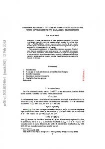
Figure 1. Fundamental relationship between an operator and its adjoint. This diagram was originally introduced to the author by Prof. John T. Wen at Rensselaer Polytechnic Institute, who attributes it to the late George Zames. 6) ( α + β )x = αx + βx. 7) ( αβ )x = α (βx ). 8) There exist scalars0 and1such that0x = 0and1x = x . Example 1 (⺢n / ⺓ n ): The most common vector space is n ⺢ , the set of real n-vectors over the reals, or more generally ⺓ n , the set of complex n-vectors over the complex field. Example 2( l n ): The set of real (respectively, complex) infinite n-tuple sequences over the real (respectively, complex) field forms a vector space. Example 3 ( Ln ): The set of continuous functions f : ⺢n → ⺢ forms a vector space. In fact, f is not required to be continuous, only measurable [4]. This class of functions includes piecewise continuous functions. Essentially, Ln includes the set of all physically realizable signals, in addition to a large number of nonphysical signals. The dimension of a vector space is defined through the notion of a basis set. A set P = { p1 , p2 , K}, is called a Hamel basis [5] for a vector space V = ( X , S ) if 1) the vectors in P are linearly independent, and 2) every vector in X can be represented by a finite linear combination of elements from P. A fundamental theorem of functional analysis is that every vector space has a Hamel basis [5, p. 211]. The notion of a Hamel basis is primarily used in analysis (see the proof of Theorem 2). In applications, it is more convenient to work with a complete basis, where infinite sums are allowed. An example is the set of complex exponentials on L2 ( −∞ , ∞ ), which are a complete basis but not a Hamel basis (since any discontinuous function in L2 ( −∞ , ∞ ) cannot be represented by a finite linear combination of complex exponentials). Definition 2: The dimension of a vector space V is the cardinality of the smallest Hamel basis for V . Example 4: The dimension of ⺢n and ⺓ n is n. The dimension of l n is ∞. The dimension of Ln is ∞. An inner product from one vector space to another vector space is defined by the following properties. Let V = ( X , S ) be a vector space, let x , y , z be elements of X, and let λ be an element of S; then ⋅, ⋅ : X × X → ⺓ is an inner product if 1) x , y = y , x ,

70

An inner product space is a vector space with an inner product. Example 5 (⺢n / ⺓ n ): The standard inner product on ⺓ n is defined as x , y = yHx =

n

∑

xi yi ,

i =1

where y H denotes the complex conjugate transpose of y. IfW is a positive definite Hermitian matrix, then another valid inner product on ⺓ n is x , y = y H Wx =

n

n

i =1

j =1

∑ ∑ wij x j yi .

Example 6 ( l n2 ): A valid inner product on infinite n-tuple sequences is a simple extension of the inner product on ⺓ n . Let x = ( x1 , x 2 , K ) and y = ( y1 , y 2 , K ) be infinite sequences with xi , yi ∈ ⺓ n . Valid inner products include the following: ∞

x, y x, y x, y

l2

= ∑ yiH xi

l2

= ∑ yiH Wxi ,

W − Hermitian

l2

= ∑ yiH xi wi ,

wi > 0.

i =1 ∞ i =1 ∞

(1)

i =1

The set of infinite n-tuple sequences such that x

l2

< ∞ is

denoted as l n2 or simply as l 2 when n is understood. Example 7 ( Ln2 ): The inner product for functions is again analogous to the inner product for l n and ⺓ n . In this case, the sum is replaced by an integral. The following are valid inner products for functions: x, y x, y x, y

L 2 ( Ω)

=∫

Ω

L 2 ( Ω)

=∫

Ω

L 2 ( Ω)

= ∫ y H ( t )x ( t )w( t ) dt , w( t ) > 0 and measurable,

y H ( t )x ( t ) dt y H ( t )Wx ( t ) dt , W − Hermitian

Ω

(2) where the integral is a Lebesgue integral [4]. The set of measurable functions on ⺓ n such that x L ( Ω) < ∞ is a valid vec2

tor space and is denoted as Ln2 (Ω ) or simply L2 when n and Ω are understood.


April 2002

A vector space V is said to be complete if all Cauchy sequences (i.e., convergent sequences) in V converge to an element of V . A Hilbert space is an inner product space that is complete. The classic example of an inner product space that is not complete is the set of continuous functions with the inner product defined in (2). For example, the Fourier series of a periodic square wave consists of an infinite sum of continuous functions. Let sn denote the first n terms in this series; then the sequence {sn } is a Cauchy sequence that converges, in the mean squared sense, to a discontinuous function. Therefore, the set of continuous functions is not a Hilbert space; however, the set of finite energy measurable functions L2 is a Hilbert space. The most commonly used Hilbert spaces are ⺢n , Cn , l 2 , and L2 . Definition 3: Let V and W be subspaces of a Hilbert space ⺘; then V is orthogonal to W, written V ⊥ W , if for all v ∈ V and all w ∈ W, v , w = 0. Definition 4: If V is a subspace of a Hilbert space⺘, then the orthogonal complement of Vin⺘ is the set

A [αu1 + βu 2] = αA [u1] + βA [u 2]. Hence, A is a linear operator over the reals. Example 10 (State Transition Matrix): The linear differential equation x& = Ax y = Cx with initial condition x (0 ) = x 0 defines a linear operator from ⺘1 = R n to ⺘ 2 = L2 [0 ,T] for ever y 0 < T < ∞ . Let A [x 0]( t ) = Ce At x 0 . Then y( t ) = A [x 0] is in L2 [0 ,T], and since

The objective of this article is to present the essential ideas behind the solution to linear operator equations.

V⊥ = {x ∈ ⺘ : ∀v ∈ V, x , v = 0}.

A [αx1 + βx 2] = αA [x1] + βA [x 2], A is a linear operator over the reals. Example 11 (Zero-State Differential Equations): The zero-initial-state linear differential equation

Definition 5: If V and W are orthogonal subspaces of a Hilbert space ⺘, then the orthogonal sum of V and W is

x& = Ax + Bu

V ⊕ W = {x ∈ ⺘ : x = v + w , v ∈ V, w ∈ W }.

with initial state x(0 ) = 0 defines a linear operator from ⺘1 = L2 [0 ,T] to ⺘ 2 = ⺢ p . The solution to this equation at time T is given by

The following lemma is proved in [3, p. 118]. Lemma 1: Let V be a closed subspace of a Hilbert space ⺘1 . Then ⺘1 = V ⊕ V⊥ .

y = Cx

y(T ) = ∫ Ce A (T − τ ) Bu ( τ ) dτ. T

0

Operators and Adjoints This note is limited to linear operators that map one Hilbert space to another. An operator A : ⺘1 → ⺘ 2 is said to be linear if for all x1 , x 2 ∈⺘1 and α , β ∈ S, where S is the field associated with ⺘1 , A ( αx1 + βx 2 ) = αA x1 + βA x 2 . Example 8 (Matrices): Let A ∈ ⺓ m×n be a complex matrix. Then A maps ⺓ n to ⺓ m and A is a linear operator over the complex field. Example 9 (Convolution): Convolution is a linear operator from⺘1 = L2 (0 ,T )to⺘ 2 = L2 (0 ,T ). Letu ∈ L2 (0 ,T )and define A [u]( t ) = ∫ u (τ )h( t − τ ) dτ t

0

A [u ( t )] = ∫ Ce A (T − τ ) Bu ( τ ) dτ. T

0

(3)

Since A [αu1 ( t ) + βu 2 ( t )] = αA [u1 ( t )] + βA [u 2 ( t )], A is a linear operator over the reals. Example 12 (Fourier Transform): The Fourier transform A [x ( t )] =

1 ∞ ∫ x ( t )e − jωt dt 2π −∞

d e f i n e s a l i n e a r o p e r a t o r f ro m ⺘1 = L2 ( −∞ , ∞ ) t o ⺘ 2 = L2 ( −∞ , ∞ ) over the complex field.

The Hilbert Adjoint Operator

for t ∈[0 ,T]. If y( t ) = A [u]( t ), then y ∈ L2 (0 ,T ) ifu ∈ L2 and h is absolutely integrable [4, p. 281]. Clearly,

April 2002

Let

A fundamental concept in linear algebra and functional analysis is the Hilbert adjoint operator. Given a linear operator


71

A : ⺘1 → ⺘ 2 , the adjoint of A , denoted A *, is an operator from ⺘ 2 to ⺘1 that satisfies Ax, y

= x, A *y

⺘2

⺓

m

= y H Ax = x , A * y

⺓

n

A *y = ∫

(4)

⺘1

for all x ∈⺘1 and all y ∈⺘ 2 . Example 13 (Matrices): Let A ∈ ⺓ m×n be a complex matrix. The adjoint of A is found by applying the definition in (4): Ax , y

Setting (7) equal to (8) gives

Ax, y

= ( A * y )H x ,

(9)

= x, A *y

⺢p

L 2 [ 0 ,T ]

,

Ax, y

T T =  ∫ x T ( τ )B T e A (T − τ )C T dτ  y 0   T T = ∫ x T ( τ )( B T e A (T −τ )C T y ) dτ

⺢p

and = ∫ x T ( τ )A *[y]( τ ) dτ. T

x, A *y L 2 ( 0 ,T )

(10)

0

Example 14 (Convolution): The adjoint of the convolution operator defined in Example 9 is defined by = x , A *[y]

T

where

A * y = ( y H A) H = A H y ⇒ A * = A H .

L 2 ( 0 ,T )

e A τ C T y( τ ) dτ.

Example 16 (Zero-State Differential Equations): Let A be the linear operator associated with the zero-state differential equation in Example 11; then the adjoint of A is defined by

which must hold for all x ∈ ⺓ n and y ∈ ⺓ m. From this equation, we see that

A [x], y

T τ =0

L 2 [ 0 ,T ]

(11)

0

, Setting (10) equal to (11) gives

where T

A [x], y

L 2 ( 0 ,T )

=∫

∫ x ( τ ) h( t − τ ) t=0 τ =0

=∫

T

T

t

τ =0

x (τ )∫

T t=τ

A *[y]( t ) = B T e A

dτy( t ) dt

h( t −τ )y( t ) dt dτ

(5)

A [x]( jω), Y ( jω) T τ =0

x ( τ ) A* [y]( τ )dτ.

(6)

By equating (5) and (6), we get that A *[y]( t ) = ∫

T σ= t

Ax, y

L 2 [ 0 , t]

L 2 [ −∞ , ∞ ]

h(σ − t )y( σ) dσ.

= x , A *y

⺢n

L 2 [ −∞ , ∞ ]

Ax, y

L 2 [ 0 ,T ]

=∫

τ =0 T

x ( t ), A *[Y ]( t )

L 2 ( −∞ , ∞ )

A *[Y ]( t ) =

Aτ

72

= ( A * y )T x .

=∫

∞ t =−∞

x ( t ) A * [Y ]( jω) dω dt .  (14) 

Setting (13) equal to (14) gives 1 ∞ e jωtY ( jω) dω, ∫ 2π ω =−∞

the inverse Fourier transform ofY ( jω). (7)

Fundamental Subspaces of a Linear Operator

(8)

The importance of the adjoint of a linear operator comes from the fundamental relationship between an operator, its adjoint, and their associated range and null spaces. The range space of an operator A : ⺘1 → ⺘ 2 is defined as

and ⺢n

,

1 ∞  ∞ ∫  ∫ x ( t )e − jωt dt  Y ( jω) dω 2π ω =−∞  t =−∞ ∞ 1 ∞ = ∫ x ( t )  ∫ω=−∞ e jωtY ( jω) dω dt 2π t =−∞ (13)

,

=  ∫ yT (τ )Ce Aτ dτ  x  τ =0  T T AT τ T  = ∫ e C y( τ ) dτ  x   τ =0

x, A *y

L 2 [ −∞ , ∞ ]

and

y ( τ )Ce x dτ T

= x ( t ), A *[Y ]( t )

=

where T

(12)

where A [[x], Y

Example 15 (State Transition Matrix): Let A be the state transition map defined in Example 10; then the adjoint of A is defined by

C y.

Example 17 (Fourier Transform): Let A be the Fourier transform operator defined in Example 12; then the adjoint of A is defined by

and x , A *[y] = ∫

(T −τ ) T


April 2002

dim (R ( A )) = dim (R ( A *)).

R ( A ) = {y ∈ ⺘ 2 : ∃x ∈ ⺘1 such that y = A x }. The null space of A : ⺘1 → ⺘ 2 is defined as N ( A ) = {x ∈ ⺘1 : A x = 0}. The objective of this section is to show that the fundamental relationship between an operator, its adjoint, and their associated range and null spaces is that illustrated in Fig. 1, namely: 1) A maps elements of⺘1 toR ( A ) ⊆ ⺘ 2 and A *maps elements of ⺘ 2 to R ( A *) ⊆ ⺘1 ; 2) ⺘1 is the orthogonal sum of N ( A ) and R ( A *) and ⺘ 2 is the orthogonal sum of N ( A *) and R ( A ); 3) The dimension of the range space of A equals the dimension of the range space of A *. The proofs of these statements are included in the following three results. Lemma 2: Let A : ⺘1 → ⺘ 2 be a bounded linear operator, where⺘1 and ⺘ 2 are Hilbert spaces. Furthermore, let R ( A ) and R ( A *) be closed. Then 1) [R ( A )]⊥ = N ( A *) and 2) [R ( A *)]⊥ = N ( A ). Pr oof : To show that [R ( A )]⊥ = N ( A *), we need to show that N ( A *) ⊆ [R ( A )]⊥ and that To show that [R ( A )]⊥ ⊆ N ( A *). N ( A *) ⊆ [R ( A )]⊥ , let y be any element in N ( A *) and let y$ be any element in R ( A ). Then there exists an x$ ∈⺘1 such that y$ = A x$ , and

Proof: We need to show that a) dim (R ( A )) ≤ dim (R ( A *)) and b) dim (R ( A *)) ≤ dim (R ( A )). To prove part a), let P = { p1 , p2 , K} be a Hamel basis for R ( A ) so dim(R ( A )) equals the cardinality of P. For each pi ∈ P, there exists a q$i ∈⺘1 such that pi = A q$i . Since ⺘1 = R ( A *) ⊕ N ( A ), there is a unique decomposition q$i = qi + ni where qi ∈R ( A *) and ni ∈ N ( A ). Therefore, pi = A qi . Let Q = {q1 ,q 2 , K}. We will show that Q is a linearly independent set, which implies that any Hamel basis of contains which implies that R ( A *) Q, dim (R ( A *)) ≥ dim (R ( A )). P is a Hamel basis for R ( A ),

The importance of the adjoint of a linear operator comes from the fundamental relationship between an operator, its adjoint, and their associated range and null spaces. which implies that all finite subsets of P are linearly independent, i.e.,

∑i ∈I ci pi

where I is a finite index set. But

y$ , y = A x$ , y = x$ , A * y

∑I

= x$ , 0 = 0,

ci pi = 0 ⇔ ⇔ ⇔

which implies that y ∈ [R ( A )]⊥ . To show that [R ( A )]⊥ ⊆ N ( A * ), let y be any element in 䉭 [R ( A )]⊥ and let x$ be any element in ⺘1 . Then y$ = A x$ is an element of R ( A ), so y$ , y = A x$ , y = 0. By definition of the adjoint, this implies that x$ , A * y = 0. Since this is true for every x$ ∈⺘1 , we must have that A * y = 0, which implies that y ∈ N ( A *). The proof that [R ( A *)]⊥ = N ( A ) is shown by similar arguments. + From Lemma 1, we therefore have the following theorem. Theorem 1: Under the hypothesis of Lemma 2: 1) ⺘1 = R ( A *) ⊕ N ( A ). 2) ⺘ 2 = R ( A ) ⊕ N ( A *). 3) dim (⺘1 ) = dim (R ( A * )) + dim ( N ( A )). 4) dim (⺘ 2 ) = dim (R ( A )) + dim ( N ( A *)). Theorem 2: Under the hypothesis of Lemma 2,

April 2002

= 0 ⇔ ci = 0, i ∈ I ,

∑ I ci Aqi = 0 A ∑ I ci qi = 0 ∑ I ci qi = 0,

where the last implication follows from the fact that ∑ I ci qi is an element of R ( A *), which is orthogonal to the N ( A ). Therefore, Q is linearly independent. The proof of part b) follows by substituting A for A * and + A * for A in the above argument. By inspecting Fig. 1, it can be seen that any element originating in ⺘1 maps to R ( A ), including elements in R ( A *). Since any element in ⺘ 2 is mapped by A *to R ( A *), it is also mapped by A A * to R ( A ). Therefore, the following lemma holds. Lemma 3: Under the hypothesis of Lemma 2: 1) R ( A ) = R ( A A *); 2) R ( A *) = R ( A * A ). Another important result that follows directly from Fig. 1 is Fredholm’s alternative [3], which is stated as Lemma 4.


73

Lemma 4: Under the hypothesis of Lemma 2, the operator equation A x = b has a solution iff b, ν = 0 for every vector ν ∈ N ( A *), i.e., b⊥ N ( A *).

Mappings and Projections In applications, it is desirable to be able to project elements of ⺘1 and ⺘ 2 to the four fundamental subspaces of A . When ⺘1 is mapped to N ( A ) or R ( A *), we would like these mappings to be projection operators. Assuming that the hypotheses of Lemma 2 are satisfied, the following paragraphs demonstrate how these operators can be constructed.

P 2 = P. Therefore, if the operator ( A A *) is invertible, the operator I − A *( A A *)−1 A projects ⺘1 onto N ( A ). Mapping from ⺘1 to R ( A ): Clearly, A maps ⺘1 to R ( A ) with no additional assumptions. Mapping from⺘1 to N ( A *): If⺘ 2 is finite dimensional with dimension m and dim(R ( A )) = p < m, then a mapping from ⺘1 to N ( A *) can be constructed by finding orthonormal vectors u p +1 , K ,u m that are orthogonal to R ( A ) and letting U 2 = (u p + 1 ,u p + 2 , K ,u m ). Then the matrix U 2 maps ⺓ ( m− p ) to N ( A *). Let Z be any onto operator from ⺘1 to ⺓ ( m− p ) ; then U 2 Z maps ⺘1 to N ( A *). Projection from⺘ 2 toR ( A ): Using arguments similar to constructing the projection from ⺘1 to R ( A ), it can be shown that if the operator A * A : ⺘1 → ⺘1 is invertible, then the operator A ( A * A )−1 A * projects ⺘ 2 ontoR ( A ). When the operator A * A is not invertible, then A SA * maps ⺘ 2 to R ( A ), where S is any invertible operator on ⺘1 . Projection from ⺘ 2 to N ( A *): Similarly, if A * A is invertible, then the operator I − A ( A * A )−1 A * projects ⺘ 2 onto N ( A *), where I is the identity operator from ⺘ 2 to ⺘ 2 . Mapping from ⺘ 2 to R ( A *): Clearly, A *maps ⺘ 2 to R ( A *) with no additional assumptions. Mapping from ⺘ 2 to N ( A ): Using arguments similar to constructing the mapping from ⺘1 to N ( A *), we get that if dim(⺘1 ) = n < ∞ , and the columns of V2 span the null space of A , then V2 Z maps ⺘ 2 to N ( A ), where Z is any onto operator from ⺘ 2 to ⺓ ( n − p ) .

A fundamental concept in linear algebra and functional analysis is the Hilbert adjoint operator. Projection from ⺘1 to R ( A *): If x ∈⺘1 , then x can be uniquely decomposed into a component in R ( A *) and a component in N ( A ). Let x = x r + x n , where x r ∈R ( A *) and x n ∈ N ( A ). Since x r ∈R ( A *), there exists an element y ∈⺘ 2 such that x r = A * y, so A x = A A * y + A x n = A A * y. If the operator A A * : ⺘ 2 → ⺘ 2 is invertible, then y = ( A A *)−1 A x , which implies that x r = A *( A A *)−1 A x . Note that P = A *( A A *)−1 A is a projection operator since P 2 = P. Therefore, if the operator( A A *) is invertible, the operator A *( A A *)−1 A projects ⺘1 onto R ( A *). When the operator A A *is not invertible, then A * SA maps ⺘1 to R ( A *), where S is any invertible operator on ⺘ 2 . Projection from ⺘1 to N ( A ): From the previous paragraph, note that xn = x − xr = x − A *( A A *)−1 A x = ( I − A *( A A *)−1 A )x ,

Characterization via Singular-Value Decomposition If the operator A is a complex m × n matrix A, then each of the fundamental spaces shown in Fig. 1 can be completely characterized by the singular-value decomposition of A[3]. If A ∈ ⺓ m×n , with rank( A) = p, then the singular-value decomposition of A is given by  Σ 0 A = ( U1 U 2 )    0 0

V1H   H  = U1ΣV1H ,  V2 

(15)

where I is the identity operator from ⺘1 to ⺘1 . Note that P = I − A *( A A *)−1 A is also a projection operator since

where Σ = diag( σ1 , K , σ p ), σ1 ≥ L ≥ σ p > 0, and U = (U1 U 2 ) and V = (V1 V2 ) are unitary matrices, i.e., H V V = I n and U H U = I m. The modification n A C of Fig. 1 for the matrix case is shown in Fig. 2. AH Cm Lemma 5: If A ∈ ⺓ m×n and if the singuN(A) = span(V2) H N(A ) = span(U2) lar-value decomposition of A is given by ⊕ ⊕ (15), then R(AH) = span(V1) R(A) = span(U1) 1) R ( A) = span(U1 ). 2) N ( AH ) = span(U 2 ). 3) R ( AH ) = span(V1 ). 4) N ( A) = span(V2 ). Figure 2. Fundamental relationship between a matrix and its Hermitian. 74


April 2002

Proof: Let y be any element of R ( A); then there exists an x ∈ ⺓ n such that y = U1ΣV1H x . Let z = ΣV1H x ; then y = U1 z , which shows that y ∈ span(U1 ). Conversely, let y be any element in the span of U1 ; then there exists some z ∈ ⺓ p such that y = U1 z . Let x = V1Σ −1 z ; then z = ΣV1H x and y = Ax , so y ∈R ( A). Since the columns of U 2 are orthonormal to the columns of U1 , and span(U ) = ⺓ m and R ( A) ⊕ N ( AH ) = ⺓ m, we must have that N ( A H ) = span(U 2 ). Similar arguments show that R ( AH ) = span(V1 ) and + N ( A) = span(V2 ). The matrix U1 is a full-rank m × p matrix and therefore defines a mapping from ⺓ p to ⺓ m, where p ≤ m. Similarly, U 2 : ⺓ m− p → ⺓ m,V1 : ⺓ p → ⺓ n , andV2 : ⺓ n − p → ⺓ n . A complete characterization of the fundamental subspaces in terms of the singular-value decomposition is depicted in Fig. 3. From Fig. 3, it is clear how to construct operators from ⺓ n and ⺓ m that map to each of the fundamental subspaces of A. The operators are defined as follows: • V2 SV2H : ⺓ n → N ( A), where S is any invertible ( n − p) × ( n − p) matrix. In particular, if S = (V2H V2 )−1 , then the operator is a projection. • V1 SV1H : ⺓ n → R ( AH ), where S is any invertible p × p matrix. In particular, if S = (V1H V1 )−1 , then the operator is a projection. • U 2 SU 2H : ⺓ m → N ( AH ), where S is any invertible ( m − p) × ( m − p) matrix. In particular, if S = (U 2H U 2 )−1 , then the operator is a projection. • U1 SU1H : ⺓ m → R ( A), where S is any invertible p × p matrix. In particular, if S = (U1H U1 )−1 , then the operator is a projection. • U1 SV1H : ⺓ n → R ( A), where S is any invertible p × p matrix. In particular, note that if S = Σ, then the mapping is simply A. • V1 SU1H : ⺓ m → R ( AH ), where S is any invertible p × p matrix. • U 2 Z : ⺓ n → N ( AH ), w h e re Z i s a n y f u l l - r a n k ( m − p) × n matrix. • V2 Z : ⺓ m → N ( A), where Z is any full-rank ( n − p) × m matrix.

Applications The objective of this section is to illustrate, through a variety of applications, the power of the concepts presented in the previous section. In particular, we will show applications to solving linear systems of equations, controllability and observability, optimal control, Kalman filtering, and modeling dynamic systems.

Linear Systems of Equations Our first application is the solution of the linear system of equations Ax = b, April 2002

(16)

Cn

A

Cn−p

V2

Cm

AH

N(A)

N(AH)

R(AH)

R(A)

V 2H

U 2H V 1H

V1

U1

Cm−p

U2

U 1H

Cp

Figure 3. Fundamental subspaces of A in terms of the singular-value decomposition. A

Cm

AH N(AH)

Cn

R(AH)

R(A)

rank(A) = N

Figure 4. Least-squares linear equations. where A ∈ ⺓ m×n , x ∈ ⺓ n , and b ∈ ⺓ m. If m = n = rank( A), then N ( A) = N ( AH ) = {0} and (16) has the unique solution x = A−1b. On the other hand, if A is not square or not full rank, then as shown in Fig. 2, either N ( A) or N ( AH ), or both, will be nontrivial. Least-Squares Solutions: Consider first the case when A is tall and full rank (i.e., m > n and rank( A) = n ). In this case, Fig. 2 reduces to Fig. 4. If b ∈R ( A), then Ax = b has a solution. Since rank( A) = n, inversion can only take place in ⺓ n . Therefore, mapping b to ⺓ n via AH gives AH b = AH Ax . Noting that AH A ∈ ⺓ n ×n is invertible, we can solve for x to obtain x = ( AH A)−1 AH b.

(17)

If b ∉R ( A), then no solution exists. The least-squares solution is defined to be 2 x$ = arg min Ax − b .

We can decompose b as b = br + bn , where br ∈R ( A) and 2 bn ∈ N ( AH ). Therefore, x$ = arg min Ax − br − bn . Since bn ⊥R ( A) and br ∈R ( A), using (17), we can minimize 2 Ax − br − bn by setting x$ = ( AH A)−1 AH br to obtain a mini2 mum value of bn . ( AH A)−1 AH (br + bn ) = ( AH A)−1 AH br implies that the least- squares solution is given by (17). The matrix A+ = ( AH A)−1 AH is called the Moore-Penrose inverse of A [6] and is an example of a pseudo-inverse of A. If


75

Cn

A AH

N(A)

Cm

R(AH)

R(A)

tion will have a zero component from N ( A); therefore, x r = V1 ζ, w h e re ζ ∈ ⺓ p . A c c o rd i n g l y, w e s e e k t h e least-squares solution to the equation AV1 ζ = b. Since b may not be in R ( AV1 ) = R ( A), we project b onto R ( A) via U1H (see Fig. 3) to get U1H AV1 ζ = U1H b. Since A = U1ΣV1H , we get Σζ = U1H b, which has a solution ζ = Σ −1U1H b, implying that x r = V1Σ −1U1H b. The solution is therefore again given by the Moore-Penrose pseudo-inverse of A:

rank(A) = n

A+ = V1Σ −1U1H .

Figure 5. Minimum-norm linear equations. the singular-value decomposition of A is A = U1ΣV , then A+ = VΣ −1U1H ∈ ⺓ n ×m. N o t e t h a t R ( A+ ) = R ( AH ) a n d N ( A+ ) = N ( AH ). Therefore, Fig. 4 could have been drawn with A+ instead of AH . Minimum-Norm Solutions: Now consider the case when A is fat and full rank (i.e., m < n and rank( A) = m). In this case, Fig. 2 reduces to Fig. 5. In this case, the equation Ax = b will have an infinite number of solutions since, if x$ is a solution, then x$ + x n will also be a solution, where x n is any vector in N ( A). Suppose that we would like the solution that has the minimum Euclidean norm; i.e., we would like to solve the optimization problem H

min x subject to:

Ax = b.

The minimum-norm solution is found by forcing the component of the solution from N ( A) to be zero. Therefore, we seek x r ∈R ( AH ) such that Ax r = b. x r ∈R ( AH ) implies that there exists a ζ ∈ ⺓ m such that x r = AH ζ; therefore, ( AAH )ζ = b. Note from Fig. 5 that ( AAH ) maps ⺓ m onto itself and is invertible; therefore, ζ = ( AAH )−1 b, which implies that x r = AH ( AAH )−1 b. The solution

Note that the standard definition of the Moore-Penrose pseudo-inverse is given as follows [6, p. 432]. If A ∈ ⺓ m×n , then the Moore-Penrose pseudo-inverse of A is the unique matrix A+ ∈ ⺓ n ×m that satisfies 1) AA+ A = A, 2) A+ AA+ = A+ , 3) ( AA+ )H = AA+ , and 4) ( A+ A)H = A+ A. It is straightforward to show that if A = U1ΣV1H is the singular-value decomposition of A, then A+ = V1Σ −1U1H satisfies the four equations listed above (use the fact that V1H V1 = I and U1H U1 = I ). Moreover, it can be shown that it is the only matrix that satisfies these equations.

Controllability Let x& = Ax + Bu be a linear system with x ∈⺢n and u ∈⺢m. The system is said to be controllable if given any initial condition x 0 , an arbitrary desired final position x f , and a finite time T > 0, there exists a control u ( t ) ∈ Lm 2 [0 ,T] that drives the system from x 0 to x f . The solution to the differential equation at time T given the initial condition x 0 is x (T ) = e AT x 0 + ∫ e A (T − τ ) Bu ( τ )dτ. T

0

Rearranging we get x (T ) − e AT x 0 = ∫ e A (T − τ ) Bu ( τ )dτ 0 = A [u], T

x = AH ( AAH )−1 b is the minimum-norm solution of the equation Ax = b. The matrix A+ = AH ( AAH )−1 is also called the Moore-Penrose inverse. Further insight about the structure of A+ can be gained from the singular-value decomposition of A. Let A = UΣV1H ; then A+ = V1Σ −1U H . Note for comparison that AH = V1ΣU H ; therefore,R ( AH ) = R ( A+ ) and N ( AH ) = N ( A+ ), which means that Fig. 5 could have been drawn with AH replaced by A+ . Minimum-Norm Least-Squares Solutions: The final case we will consider is the general problem shown in Fig. 2, where rank( A) = p < min( m, n). In this case, the solution is most easily derived using Fig. 3, where it can be seen that the solution can be decomposed into two problems: a least-squares solution from ⺓ p to ⺓ m and a minimum-norm solution from ⺓ n to ⺓ p . From Fig. 3, we see that the minimum-norm solu76

n where A is defined in (3) and maps ⺘1 = Lm 2 [0 ,T] to ⺘ 2 = ⺢ . Clearly, to allow x f = x (T ) to be arbitrarily assigned for any initial condition x 0 requires that R ( A ) = ⺢n , in which case n Fig. 1 reduces to Fig. 6. Since A : Lm 2 [0 ,T] → ⺢ , the system will be controllable if and only if rank( A ) = rank( A A *) = n. To derive the standard controllability criteria, we solve for the minimum-norm solution to this operator equation. Accordingly, let u ∈R ( A *); then u = A * ζ, where ζ ∈⺢n and A * is given in (12). Therefore, ζ satisfies ( A A *)ζ = x f − e AT x 0 , where the matrix ( A A *) has dimension n × n. By Sylvester’s rank inequality [3, p. 250], if rank( A ) = n, then ( A A *) has rank equal to n and is hence invertible. Therefore, there exists a control signal in Lm 2 [0 ,T] that drives the system from any initial condition x 0 to any final configuration x f if and only if the rank of the matrix


April 2002

( A A *) = ∫ e A (T − τ ) BB T e A T

T

(T − τ )

dτ

0

is equal to n. The matrix in (18) is called the controllability Grammian. Using the Cayley-Hamilton theorem [6], it is straightforward to show that the controllability Grammian has rank n if and only if the matrix (B

AB

A B ⋅⋅⋅ A 2

n −1

Lm 2 [0,T]

(18)

A A*

N(A) Rn

⊕ R(A*)

R(A)

B)

has rank n, which is the standard controllability criterion [7].

Figure 6. Fundamental subspaces for controllability.

Optimal Control

min u

Rn

R(A*)

The constraint could also be written as xf = e x0 + ∫ e tf

A(t−τ )

0

A* N(A*)

L2

subject to: x& = Ax + Bu x (0 ) = x 0 x( tf ) = x f .

At

Lp2[0,T]

A

Consider the optimal control problem

R(A)

Figure 7. Fundamental subspaces for observability.

Bu ( τ )dτ.

Let A [u] = ∫ e A ( tf − τ ) Bu ( τ )dτ be the linear operator de0 fined in Example 11; then the objective is to find the minimum-norm solution to the linear operator equation

finite period of time [0 ,T]. As discussed in Example 10, the output y( t ) is given by the equation

tf

A [u] = x f − e Atf x 0 .

(19)

In the previous section, we showed that the minimum-norm solution is given by u = A * ζ, where ζ satisfies A A * ζ = x f − e Atf x 0 and where A A * is the controllability Grammian given in (18). If the system is controllable, then A A * is invertible, which implies that the minimum-norm control is given by u ( t ) = A * ( A A *) T

= eA

( tf − t )

−1

(x

f

− e Atf x 0

)

C T  ∫ Ce A ( tf − τ ) e A  0 tf

T

C dτ  

( tf − τ ) T

−1

(x

f

)

− e Atf x 0 .

䉭

y( t ) = Ce At x 0 = A [x 0]( t ), where A : ⺢n → LP [0 ,T]. To allow x 0 to be uniquely determined requires that the dimension of R ( A *) be equal to n, in which case Fig. 1 reduces to Fig. 7, where A *is given by (9). In this case, y( t ) ∈R ( A ), and therefore no information is lost by mapping y to R n via A * to obtain A *[y] = A * A [x 0]. The n × n matrix A *A = ∫

e A τ C T Ce Aτ dτ T

is called the observability Grammian of system (20). By Lemma 3,R ( A * A ) = R ( A *), which implies that system (20) is observable if and only if rank( A * A ) = n. Using the Cayley-Hamilton theorem [6], it is straightforward to show that the observability Grammian has rank n if and only if the matrix

(C

Observability Let x& = Ax y = Cx

T τ =0

T

AT C T ⋅⋅⋅ A( n −1 )T C T

)

T

has rank n, which is the standard observability criterion [7]. (20)

Optimal, Unbiased Estimation Consider the dynamic system

be a linear system with x ∈⺢n , y ∈⺢ p , and initial condition x (0 ) = x 0 . The system is said to be observable if the initial condition x 0 is uniquely identified by the output y( t ) over a

April 2002


x& = Ax , x ( t 0 ) = x 0 y = Cx + ξ,

(21)

77

T T x$ 0 =  ∫ e A τ C T Ce Aτ dτ  = 0 τ  

y

−1 T

∫τ = 0

e A τ C T y( τ )dτ. T

x Since the covariance of the noise is identity, this is also the minimum variance estimate [3].

Dynamics of Constrained Mechanical Systems

L

Mechanical systems are often modeled using Lagrangian or Hamiltonian formulations. An alternative method, presented in [8], uses Gauss’s principle and the techniques developed in these notes. The technique is best illustrated via an example. Following [8], let x = ( x , y )T be the coordinates of a point-mass with mass m that is subjected to a force F = ( Fx , Fy )T . The “unconstrained” acceleration of the point x is given by

g m Figure 8. Point-mass suspended by massless rod.

where ξ is a zero mean Gaussian process with covariance equal to the p × p identity matrix. The objective is to develop an unbiased estimate of x 0 from measurements of y( t ) over the interval [t 0 , t f ]. The solution to the differential equation (21) is y( t ) = Ce At x 0 + ξ( t ) = A [x 0] + ξ( t ), where A : ⺢n → L p [t 0 , t f ] is given in Example 10. As shown in the previous example, if the system is observable, then rank( A ) = rank( A * A ) = n. The objective is to find a linear operator K : L p [t 0 , t f ] → ⺢n such that

a = M −1 F where M = mI 2 and a is the unconstrained acceleration. Alternatively, if the point-mass is constrained, then the actual acceleration will differ from the unconstrained acceleration. Suppose, for example, that the point-mass is constrained to be at the end of a massless rod of length L rigidly suspended from the point (0 ,0 )T , as in Fig. 8. In this case, the point-mass satisfies the constraint φ( x ) = x 2 + y 2 − L2 = 0. Differentiating ϕ twice, we conclude that the actual acceleration of the point-mass must satisfy the constraint A( x )x&& = b( x , x& ), where A( x ) = ( x , y ) and b( x , x& ) = − x& 2 − y& 2 . Gauss’s principle states that the acceleration of the point-mass will satisfy the following minimization problem:

x$ 0 = K [y] is an unbiased estimate of x 0 ; i.e.,

min ( x&& − a )T M ( x&& − a ) subject to: Ax&& = b.

E {x$ 0 } = x 0 . Therefore, we have

Alternatively, we can write

(

E {x$ 0 } = E {K [y]} = E {K [A [x 0] + ξ]} = E {( KA )[x 0] + K ξ} = ( KA )[x 0] + E {K ξ} = ( KA )[x 0].

min M 1 / 2 x&& − M 1 / 2 a subject to: AM

−1 / 2

) (M T

(M

1 / 2 &&

Note that KA : ⺢ → ⺢ is an n × n matrix. If KA = I , then $ E {x 0 } = x 0 , which implies that x$ 0 is an unbiased estimate. Therefore, K is a left inverse operator of A . From Fig. 1 it is clear that such an operator is

subject to:

2

( AM )ξ = b − Aa, −1 / 2

which is the standard minimum-norm least-squares problem discussed earlier in this section. The solution is therefore given by

(

ξ = AM −1 / 2

Therefore, an unbiased estimate of x 0 is

78

)

)

Letting ξ = M 1 / 2 x&& − M 1 / 2 a gives

n

K = ( A * A )−1 A *.

x − M 1/ 2a

x = b.

min ξ

n

1 / 2 &&


) (b − Aa ), +

April 2002

[2] D.G. Luenberger, Optimization by Vector Space Methods. New York: Wiley, 1969.

or alternatively,

(

x&& = a + M −1 / 2 AM −1 / 2

[3] T.K. Moon and W.C. Stirling, Mathematical Methods and Algorithms. Englewood Cliffs, NJ: Prentice Hall, 2000.

) (b − Aa ). +

[4] F. Jones, Lebesgue Integration on Euclidean Space. Boston, MA: Jones and Bartlett, 1993.

For the point-mass shown in Fig. 8, we get

[5] E. Kreyszig, Introductory Functional Analysis. New York: Wiley, 1978. [6] P. Lancaster and M. Tismenetsky, The Theory of Matrices, 2nd ed. San Diego, CA: Academic, 1985.

 0  1 x x&& =   + 2   − x& 2 − y& 2 + gy .  −g  L  y 

(

)

[7] W.J. Rugh, Linear System Theory, 2nd ed. Englewood Cliffs, NJ: Prentice Hall, 1996. [8] F.E. Udwadia and R.E. Kalaba, Analytical Dynamics: A New Approach. New York: Cambridge Univ. Press, 1996.

Conclusions This lecture note has presented a unified approach to bounded linear operator equations on Hilbert spaces. We have shown that linear operators can be completely understood via the diagram shown in Fig. 1, which represents the fundamental subspaces of a bounded linear operator. We have also shown a number of applications of the underlying theory. The objective of these notes has been to present the fundamentals in a pedagogically clear manner, in the hope that they will enable readers to successfully apply the concepts to their own problems.

References [1] G.C. Goodwin, S.F. Graebe, and M.E. Salgado, Control System Design. Englewood Cliffs, NJ: Prentice Hall, 2001.

April 2002

Randal W. Beard received a B.S. in electrical engineering from the University of Utah in 1991 and an M.S. in electrical engineering in 1993, an M.S. in mathematics in 1994, and a Ph.D. in electrical engineering in 1995, all from Rensselaer Polytechnic Institute, Troy, NY. Since 1996, he has been an Assistant Professor in the Electrical and Computer Engineering Department at Brigham Young University, Provo, UT. In 1997 and 1998, he was a summer faculty fellow at the Jet Propulsion Laboratory, California Institute of Technology. His research interests include coordinated control of multiple-vehicle systems and nonlinear control. He is a member of the IEEE, AIAA, and Tau Beta Pi.


79