Evolution Strategies Learned with Automatic Termination Criteria Abdel-Rahman Hedar and Masao Fukushima Department of Applied Mathematics and Physics Graduate School of Informatics, Kyoto University, Kyoto 606-8501, JAPAN email: {hedar,fuku}@amp.i.kyoto-u.ac.jp
Abstract— Although several attempts have been made to modify the original versions of Evolutionary Algorithms (EAs), they are not learned with automatic termination criteria. In general, EAs cannot decide when or where they can terminate. In this paper, we modify Evolution Strategies (ESs) with new termination criteria. The proposed method is called ESs Learned with Automatic Termination (ESLAT). In the ESLAT method, a so-called Gene Matrix (GM) is constructed to equip the search process with a self-check to judge how much exploration has been done. Moreover, an especial mutation operation called “Mutagenesis” is defined to achieve more efficient and faster exploration process. The computational experiments show the efficiency of the ESLAT method. Keywords—Evolution Strategies, Evolutionary Algorithms, Heuristics, Global Optimization, Termination Criteria, Mutagenesis
I. I NTRODUCTION Evolutionary Algorithms (EAs) constitute one of the main tools in computational intelligence area [4], [13]. Achieving practical versions of EAs is highly needed to confront the rapid growth of many applications in science, engineering and economics [1], [13]. Nowadays, there is a great interest to improve the evolutionary operators which go further than modifying their genetics to use the estimation of distribution algorithms in generating the offspring [16], [17]. However, EAs still have no automatic termination criteria. Actually, EAs cannot decide when or where they can terminate and usually a user should prespecify a maximum number of generations as termination criteria. An intelligent search method should perform a wide exploration with a deep exploitation. Moreover, it should also have its strategies to check the progress of its main processes; exploration and exploitation. This can equip the search method with automatic termination criteria. In this paper, a new version of Evolution Strategies (ESs) called Evolution Strategies Learned with Automatic Termination (ESLAT) is proposed. In the ESLAT method, the standard ESs are equipped with automatic termination criteria. Moreover, new elements are introduced to achieve a better performance of ESs. Our goal is to construct an intelligent method which seeks optimal or near-optimal solutions of a given objective function. Abdel-Rahman Hedar is also affiliated with the Department of Computer Science, Faculty of Computer and Information Sciences, Assiut University, EGYPT (email:
[email protected]).
This problem can be expressed as follows. min f (x),
x∈X
(P)
where f is a real-valued function defined on the search space X ⊆ Rn with variables x ∈ X. Several versions of EAs have been proposed to deal with this problem, see [6], [8], [16] and reference therein. This problem has also been considered by other heuristics than EAs, see [9], [10] and references therein. Many applications in different areas of computer science, engineering, and economics can be expressed or reformulated as Problem (P ) [1], [5]. The ESLAT method is composed by modifying ESs with some directing strategies. First, an exploration and exploitation scheme is invoked to equip the search process with automatic termination criteria. Specifically, a matrix called Gene Matrix (GM) is constructed to represent sub-ranges of the possible values of each variable. The role of GM is to assist the exploration process in two different ways. First, GM can provide the search with new diverse solutions by applying a new type of mutation called “mutagenesis”. Mutagenesis operator alters some survival individuals in order to accelerate the exploration process. In addition, GM is used to let ESLAT know how far the exploration process has gone in order to judge a termination point. Then, a final intensification process can be started in order to refine the elite solutions obtained so far. Moreover, some promising children are detected to be guided to nearest local minima. The numerical results shown later indicate that the proposed ESLAT method is competitive with some other versions of ESs. In the next section, we present the principles of Evolution Strategies. In Section 3, we highlight the main components of the ESLAT method. In Section 4, we discuss numerical experiments with the ESLAT method. Finally, the conclusion makes up Section 5. II. E VOLUTION S TRATEGIES Evolution Strategies (ESs) are a major class of evolutionary algorithms (EAs) [2], [3]. Improving existing ESs has been fascinating many researchers by modifying their operators, see [6], [25] for instance. ESs start with a population of candidates of µ trial solutions. At each iteration (generation), ESs update each individual in the population using some control parameters called strategy parameters. This updating process is remarked as the ES-mutation operation. Beside this
mutation operation, ESs may utilize a recombination operation by mating ρ parents to reproduce a new child. At the end of each generation, ESs maintain only µ individuals out of λ generated children with or without their parents. This process is known as the selection operation. There are two main selection schemes in ESs; “+” and “,” selection schemes which compose the well-known ESs versions; (µ/ρ+λ)-ES and (µ/ρ,λ)-ES. The “,” selection scheme is a truncation selection mechanism in which the parents have no chance to survive. Contrary to “,” selection, the “+” selection scheme give the parents a chance to contribute in the next generation based on the elitism. The main operation in ESs is the mutation which updates each individual x in a currant population P by adding a displacement ∆x based on a given normal (Gaussian) distribution N (ζ, σ) with the probability density function (∆x−ζ)2 1 √ e− 2σ2 . (1) σ 2π The mean ζ is usually set to zero [3] but some ESs versions utilize some biased mutation with ζ differs than zero [14]. The variance σ is called the strategy parameter and it can be adjusted through different rules, see [2], [3]. A formal algorithm of ESs is given in the following. Algorithm 2.1: (µ/ρ +’ λ)-ES Algorithm 1. Initialization. Create the initial population P0 = {(xi , σ i , F (xi )), i = 1, . . . , µ}, and set the generation counter g := 0. 2. Main Loop. Repeat the following steps (2.1) – (2.3) for j = 1, . . . , λ. 2.1 Recombination. Choose ρ parents p1 , . . . , pρ from Pg , and calculate the mated child
p(∆x) =
In the (µ/ρ,λ)-ES, the selection mechanism is a strict Darwinian selection in which all parents are discarded whether they are good or bad. We think this is not an optimal selection mechanism since some good solutions may be lost if all parents are discarded. In the (µ/ρ+λ)-ES, the µ best individuals out of the parents and offspring only survive to the next generation. We think this is also not an optimal section mechanism since it may lead to immature convergence and the diversity may be lost. Therefore, we compose a new operation called “mutagenesis” in order to alter some survival individuals to new unexplored areas which helps in maintaining the diversity. Moreover, this new operation works within the “+” selection mechanism in order to maintain the elitism. Termination criteria are the main drawback of ESs and EAs in general. They are not equipped with automatic termination criteria. Actually, EAs may obtain an optimal or near-optimal solution in an early stage of the search, but they were not learned enough to judge whether they could terminate. So that the ESLAT is built with termination measures which can check the progress of the exploration process through successive generations. Then, an exploitation process starts to refine the best candidates obtained so far in order to achieve faster convergence. In designing ESLAT, we have considered the abovementioned remarks. The standard ESs algorithm is modified with the below-mentioned components to compose the ESLAT method. •
(ˆ xj , σ ˆ j ) = recombine(p1 , . . . , pρ ). 2.2 Mutation. Calculate the mutated child (˜ xj , σ ˜ j ) = mutate(ˆ xj , σ ˆ j ). 2.3 Fitness. Evaluate the fitness function F˜ j = F (˜ xj ). 3. Children Pool. Collect all generated children in Cg = {(˜ xj , σ ˜ j , F˜ j ), j = 1, . . . , λ} 4. Selection. Choose the next generation Pg+1 from ( select(Cg ) for (µ/ρ,λ)-ES version, Pg+1 = select(Pg ∪ Cg ) for (µ/ρ+λ)-ES version. 5. Termination. If the termination conditions are satisfied, then stop. Otherwise, set g := g + 1 and go to Step 2. III. E VOLUTION S TRATEGIES L EARNED WITH AUTOMATIC T ERMINATION In this section, a new modified version of ESs called Evolution Strategies Learned with Automatic Termination (ESLAT) is presented. Before presenting the details of ESLAT, we highlight some remarks on ESs as motivations for proposing ESLAT.
•
Gene Matrix and Termination. Each individual x in the search space consists of n variables or genes since ESs use the real-coding representation of individuals. The range of each gene is divided to m sub-ranges in order to check the diversity of each gene values. The gene matrix GM is initialized to be an n × m zero matrix in which each entry of each row refers to a sub-range of the corresponding gene. While the search is processing, the entries of GM is updated from zeros to ones if new values for genes are generated within the corresponding sub-ranges. Figure 1 shows an example of GM in two dimensions. In this figure, the range of each gene is divided into 5 sub-ranges, and GM has three zero-entries corresponding to three sub-ranges in which there is no individual generated. After having a GM full with ones, the search is learned that an advanced exploration process has been achieved. However, the search is not stopped at that moment and will continue to give a chance to the recently chosen subranges to be wildly explored with the help of recombination operation. Therefore, GM is used to equip the search process with practical termination criteria. Moreover, GM assists in providing the search with diverse solutions as we will show below. Mutation. The mutated children are generated as in the standard ESs [2], [3]. Therefore, a mutated child (˜ x, σ ˜ ) is obtained from a parent (ˆ x, σ ˆ ), where the i-th component
x2 p1 p2 µ
1 1 1 1
GM =
0 1
1 0 1 0
¶ A Recombined Child
p4
x1 Search Space Fig. 1.
p3
Gene Matrix
An example of the Gene Matrix in R2 .
Parents Fig. 2.
An example of the recombination operation.
x2
x2
of the mutated child (˜ x, σ ˜ ) is given as 0
•
σ ˜i = σ ˆi eτ N (0,1)+τ Ni (0,1) , (2) x ˜i = x ˆi + σ ˜i Ni (0, 1), (3) p √ √ where τ 0 ∝ 1/ 2n and τ ∝ 1/ 2 n, and the proportional coefficients are usually set to one. Mutagenesis. In order to accelerate the exploration process, a more artificial mutation operation called “mutagenesis” is used to alter the Nw worst individuals selected for the next generation. Specifically, a zero-position in GM is randomly chosen, say the position (i, j), i.e., the variable xi has not been yet taken any value in the j-th partition of its range. Then, a random value for xi is chosen within this partition to alter one of the chosen individual for mutagenesis. A formal procedure for mutagenesis is given as follows.
∗ ∗
µ GM = (a) Fig. 3.
Recombination. The recombination operation has an exploration tendency, therefore, it is not applied for all parents. Specifically, it is applied with probability pr ∈ [0, 1). The mechanism in the recombination operation is to choose randomly ρ parents p1 , . . . , pρ form the current generation. A recombined child x ˆ is calculated to have ρ (ρ ≤ n) partitions, and each partition is inherited from one parent. As an example, Figure 2 shows that 4 parents p1 , p2 , p3 and p4 partitioned into 4 partitions at same positions (after the first, third and sixth genes). Then, a recombined child is generated to inherit its first partition from p3 , its second partition from p1 , its third partition from p4 and its last partition from p2 . The following procedure describes the ESLAT recombination operation precisely. Procedure 3.2: Recombination(p1 , . . . , pρ )
1 1
x1
¶x1
“ ∗ ” = a recombined child
(b)
The role of recombination operation and GM.
1. If ρ > n then return, otherwise go to Step 2. 2. Partition each parent into ρ partitions at the same positions, i.e., pj = [X1j X2j . . . Xρj ], j = 1, . . . , ρ. 3. Order the set {1, 2, . . . , ρ} randomly to be {o1 , o2 , . . . , oρ }. 4. Calculate the recombined child x = o [X1o1 X2o2 . . . Xρ ρ ], and return.
Procedure 3.1: Mutagenesis(x, GM) 1. If GM is full then return, otherwise go to Step 2. 2. Choose a zero-position (i, j) in GM randomly. −li 3. Update x by setting xi = li + (j − r) uim , where r is a random number from (0, 1), and li , ui are the lower and upper bound of the variable xi , respectively. 4. Update GM by setting GMij = 1, and return. •
1 1
•
It is noteworthy that the ESLAT recombination can be considered a general form of well-known crossover types called “single point crossover” and “two point crossover” [18]. Actually, this type of recombination is defined to support the ESLAT exploration process. Specifically, there no information related to different sub-ranges of disjoint variables is saved in GM in order to escape from the complexity of high dimensional problems. Therefore, there is a possibility of having misguided termination of exploration process as in the example shown in Figure 3(a). However, invoking such recombination operation as in Procedure 3.2 can easily outperform such drawback as shown in 3(b). Moreover, the numerical simulations presented in Section IV show that the ESLAT exploration process can discover the search space widely. Selection. The ESLAT selection operation uses the standard ESs “+” selection to choose the survival individuals from the generation Pg into its proceeding one Pg+1 . However, the mutagenesis operation is used to alter some of them in order to drive the search into new diverse areas.
Intensification Process. After computing all children in each generation, ESLAT gives a chance to two characteristic children to improve themselves by apply a local search starting from each of them. These characteristic children are the child who can update the best solution found so far, and the child with the highest difference of the objective function between a parent and his child in the currant generation. We call these characteristic children “the best child” and “the most promising child”, respectively. The intensification process of improving these characteristic children lets ESLAT behave like a so-called “Memetic Algorithm” [20] in order to achieve faster convergence [23], [24]. After finishing the exploration process, another intensification process is started by applying an efficient local search method to refine the best solutions obtained so far. Specifically, a derivativefree local search method is applied starting from each point out of the Nelitet best ones obtained so far. This intensification process can overcome the slow convergence of EAs at the end stage and helps to avoid the EAs wandering around the optimal solution. The formal algorithm of the ESLAT method is stated below. Algorithm 3.3: ESLAT Algorithm 1. Initialization. Create an initial population P0 = {(xi , σ i , F (xi )), i = 1, . . . , µ}, construct the gene matrix GM. Choose the recombination probability pr ∈ [0, 1], set values of; ρ, Nw and Nelitet , set ν := λ/µ, and set the generation counter g := 0. 2. Main Loop. Repeat the following steps (2.1) – (2.3) from j = 1, . . . , µ. 2.1 Recombination. Generate a random number χ ∈ [0, 1]. If χ > pr , choose a parent (ˆ xj , σ ˆj ) from Pg and go to Step 2.2. Otherwise, choose ρ parents p1 , . . . , pρ from Pg , and calculate the recombined child (ˆ xj , σ ˆ j ) using Procedure 3.2. 2.2 Mutation. Use the individual (ˆ xj , σ ˆ j ) to j,k j,k calculate the mutated children (˜ x ,σ ˜ ), k = 1, . . . , ν, as in equations (2) and (3). 2.3 Fitness. Evaluate the fitness function F˜ j,k = F (˜ xj,k ), k = 1, . . . , ν. 3. Children Pool. Collect all generated children in Cg = {(˜ xj,k , σ ˜ j,k , F˜ j,k ), j = 1, . . . , µ, k = 1, . . . , ν} 4. Local Search. Apply a local search to improve the best child (if exists) and the most promising child in Cg . 5. Termination. If n generations have passed after getting a full GM, then go to Step 8. Otherwise, go to Step 6. 6. Selection. Choose the best µ individuals from Pg ∪ Cg to compose the next generation Pg+1 . Update the gene matrix GM. 7. Mutagenesis. Apply Procedure 3.1 to alter the Nw worst individuals in Pg+1 , and set g := g+1, and go to Step 2. 8. Intensification. Apply a local search method starting from each solution from the Nelite elite
TABLE I ESLAT PARAMETER S ETTING
•
Parameter µ λ ρ pr σ0 σmin σmax m Nw Nelite
Definition Population size No. of mutated children No. of mated parents Probability of recombination operation Initial mutation parameter Min. allowed for σ components Max. allowed for σ components No. of GM columns No. of individuals used by mutagenesis No. of starting points for intensification
Value 15 7µ min{n, 5} 0.5 (3,. . . ,3) 1e–4 0.5d 30 5 1
ones obtained in the previous search stage. IV. N UMERICAL E XPERIMENTS Algorithm 3.3 was programmed in MATLAB and applied to 23 well-known test functions [25], [26], see the Appendix. The functions can be classified into two classes; the functions of low dimensional functions (f14 -f23 ) and the functions of high dimensional functions (f1 -f13 ). For each function, the ESLAT MATLAB code was run 50 times with different initial populations. The main results are reported in Tables III, IV and V as well as in Figures 4 and 5. Before discussing these results, we summarize the setting of the ESLAT parameters. First, the search space for Problem P is defined as [L, U ] = {x ∈ Rn : li ≤ xi ≤ ui , i = 1, . . . , n} , with diameter d := max1≤i≤n (ui − li ) . In Table I, we summarize all parameters used in the ESLAT algorithm with their assigned values. These chosen values are based on the common setting in the literature or based on our numerical experiments. In the ESLAT algorithm, we used the scatter search diversification generation method [15], [11] to generate the initial population P0 . In that method, the interval (ui − li ) of each variable is divided into 4 sub-intervals of equal size. New points are generated to be added to P0 as follows. 1) Choose one sub-interval for each variable randomly with a probability inversely proportional to the number of solutions previously chosen in this sub-interval. 2) Choose a random value for each variable that lies in the corresponding selected sub-interval. To avoid an inefficient small mutation, the strategy parameter σ is bounded below by the value σmin as it is recommended in [22]. Moreover, σ is also bounded above by the value σmax to avoid too big mutations which may lead the search outside the search space especially for problems with small search spaces. We tested three mechanisms for local search method in the intensification process based on two methods: Kelley’s modification [12] of the Nelder-Mead (NM) method [21], and a MATLAB function called “fminunc.m”. These mechanisms are 1) method1 : to apply 10n iterations of Kelley-NM method, 2) method2 : to apply 10n iterations of MATLAB fminunc.m function, and
TABLE II R ESULTS OF L OCAL S EARCH S TRATEGIES
f f18 f19 f15 f2 f9
n 2 3 4 30 30
Initials f¯ 46118 –0.9322 8.8e+5 2.2e+20 551.7739
f14 60
40
Local Search Strategy f¯method1 f¯method2 f¯method3 371.3246 23.8734 13.0660 –2.6361 –2.8486 –3.6695 1998.5 0.0120 0.0309 1.2+e19 1.1e+13 340.6061 256.0628 91.5412 193.4720
20
0
−20
−40
−60 −60
3) method3 : to apply 5n iterations of Kelley-NM method, then apply 5n iterations of MATLAB fminunc.m function. Five test functions were chosen to test these three mechanisms as in Table II. One hundred random initial points were generated in search space of each test function. Then, the three local search mechanisms were applied to improve the generated points, and the average results are reported in Table II. The last mechanism “method3 ” could improve the initials significantly, and it is better than the other two mechanisms. Therefore, ESLAT invokes “method3 ” for local search in Step 4 of Algorithm 3.3. Moreover, method3 was used with bigger numbers of iterations as a final intensification method in Step 8 of Algorithm 3.3. Extensive numerical experiments were done to show the efficiency of ESLAT and to give an idea about how it works. First, preliminary experiments given in Figures 4 and 5 show the role of exploration and automatic termination using GM. Graphs in Figure 4 show the distributions of all generated solutions during the ESLAT exploration process (without the final intensification) of all two dimensions test functions (f14 , f16 , f17 and f18 ). This figure shows that the ESLAT exploration process can discover the search space widely. In Figure 5, the solid vertical lines refer to the generation number of having a full GM, while the dotted vertical lines refer to the generation number of terminating the exploration process just before applying the final intensification. The ESLAT code continued running after reaching the dotted lines without applying the final intensification in order to check efficiency of the automatic termination. The graphs in Figure 5 show that no much improvement achieved after the dotted lines. However, using the final intensification (Step 8 in the ESLAT algorithm) can accelerate the convergence in the final stage instead of letting the algorithm running for several generation without much significant improvement. It is noteworthy that using GM in the termination criteria seems to be affected by the curse of dimensionality since its performance with higher dimensional problems is relatively worse than that of lower ones. ESLAT was compared with three other ESs versions; Canonical Evolution Strategies (CES), Fast Evolution Strategies (FES) [25], and Covariance Matrix Adaptation Evolution Strategies (CMA-ES) [6]. These comparisons are reported in Tables III, IV and V containing the mean and the standard division (SD) of the best solutions obtained for each function as measures of solution qualities, and the average number of function evaluations as measures of solution costs. These results were obtained out of 50 runs. Moreover, t-tests [19]
−40
−20
0
20
40
60
f16 5 4 3 2 1 0 −1 −2 −3 −4 −5 −5
0
5
f17 15
10
5
0 −5
0
5
10
f18 2 1.5 1 0.5 0 −0.5 −1 −1.5 −2 −2
Fig. 4.
−1.5
−1
−0.5
0
0.5
1
1.5
2
Distributions of Generated Solutions
for solution qualities are also reported to show the significant differences between the compared methods. The FEP results reported in Tables IV are taken from their original paper [25]. The CMA-ES results reported in Tables V are generated by running its code downloaded from its inventor homepage (http://www.bionik.tu-berlin.de/user/niko/index.html). The results shown in Table III aim at showing how much the new components in the ESLAT method, especially the termination criteria, help improve the efficiency of the algorithm. So, the CES algorithm has been run under the same parameters setting as in the ESLAT algorithm and with a termination condition of reaching a maximum number of
TABLE III S OLUTION Q UALITIES FOR ESLAT AND CES Solution Qualities f f1 f2 f3 f4 f5 f6 f7 f8 f9 f10 f11 f12 f13 f14 f15 f16 f17 f18 f19 f20 f21 f22 f23
n 30 30 30 30 30 30 30 30 30 30 30 30 30 2 4 2 2 2 3 6 4 4 4
ESLAT Mean SD 2.0e–17 2.9e–17 3.8e–5 1.6e–5 6.1e–6 7.5e–6 0.78 1.64 1.93 3.35 2.0e–2 0.14 0.39 0.22 –2.3e+15 5.7e+15 4.65 5.67 1.8e–8 5.4e–9 1.4e–3 4.7e–3 1.5e–12 2.0e–12 6.4e–3 8.9e–3 1.77 1.37 8.1e–4 4.1e–4 –1.0316 9.7e–14 0.398 1.0e–13 3 5.8e–14 –3.8628 2.9e–13 –3.31 3.3e–2 –8.49 2.76 –8.79 2.64 –9.65 2.06
t-test for Solution Qualities
CES Mean SD 1.7e–26 1.1e–25 8.1e–20 3.6e–19 337.62 117.14 2.41 2.15 27.65 0.51 0 0 4.7e–2 0.12 –8.0e+93 4.9e+94 13.38 43.15 6.0e–13 1.7e–12 6.0e–14 4.2e–13 1.46 3.17 2.40 0.13 2.20 2.43 1.3e–3 6.3e–4 –1.0310 1.2e–3 0.401 3.6e–3 3.007 1.2e–2 –3.8613 1.2e–3 –3.24 5.8e–2 –5.72 2.62 –6.09 2.63 –6.42 2.67
function evaluations equal to the average number obtained in the ESLAT experiments. In other words, both ESLAT and CES codes are terminated at almost the same number of function evaluations. The results in Table III show that the ESLAT was only outperformed by CES on five problems f1 , f2 , f7 , f10 and f11 , and for almost all of these problems the ESLAT could reach very close to the global minima. It is also shown that ESLAT is robust and can reach global minima or at least very close to them in many test problems. It is noteworthy that we do not use any methodology to maintain the search within certain feasible regions in the ESLAT and CES codes, which may explain why they obtained unexpected solutions for problem f8 which lie outside the search space and have function values lower than the known values. For the results in Tables IV, we can conclude that ESLAT outperforms FES on 12 problems in terms of solution qualities and the latter is much expensive than ESLAT. Moreover, ESLAT still outperforms FES in terms of solution costs on another 6 problems for which both ESLAT and FEP are neutral in terms of solution qualities. For the rest of test problems (5 test problems), we cannot conclude any judgement since ESLAT outperforms FEP in terms of solution costs and the latter outperforms in terms of solution qualities. Another observation on the results in Table IV is concerned with the termination criteria which are automatically set in the ESLAT but problem-dependent in FES. The number of generations in FEP must be provided by the user and this is questionable since there is no rule a user can follow to detect this number in advance. For example, this number is set equal to 7,500 for function f5 and equal to 750 for functions f10 , f12 and f13 , although all of them have dimension 30 and f5 is a uni-modal function while the others have serval local minima. There are several attempts to modify the strategy parameters
t-value ESLAT – CES 4.9 16.8 –20.3 –4.4 –53.7 1.0 9.7 – –1.4 23.6 2.1 –3.2 –130.0 –1.1 –3.5 –3.5 –5.9 –4.1 –8.8 –7.4 –5.1 –5.1 –6.8
Significant Method at level 0.05
CES CES ESLAT ESLAT ESLAT – CES – – CES CES ESLAT ESLAT – ESLAT ESLAT ESLAT ESLAT ESLAT ESLAT ESLAT ESLAT ESLAT
of ESs, and the most common one is what we have used in Equations (2) and (3). One of the most promising and efficient of the recent modifications is the CMA-ES [7], [6]. In the following we discuss our results against the CMA-ES, using the figures shown in Tables V. The percentages between parentheses in Table V show the success rate of reaching within gap of 10−3 fare from the global minima function values. It does not seem to make fair comparisons between ESLAT and CMA-ES since they have different termination conditions. First, CMA-ES is one of the most reliable and fast versions of ESs and its general performance is better and cheaper than ESLAT for the high dimensional functions especially for uni-model functions (f1 , . . . , f7 ). However, the CMA-ES’s superior performance deteriorates for the low dimensional functions. Moreover, it seems that the CMA-ES was sometimes trapped in local minima even for some easy functions like f18 . As shown in Figure 6, the global minimum of f18 lies in a widespread valley. Therefore, it is not difficult for a search method with an efficient exploration process to reach the global minimum. However, CMA-ES failed to reach the global minimum for 22% of trails. Actually, CMA-ES cannot outperform ESLAT for any of the low dimensional function in terms of solution qualities or in the success rate, although it is still cheaper for some of these functions. V. C ONCLUSIONS A new version of ESs called Evolution Strategies Learned with Automatic Termination (ESLAT) has been proposed in order to achieve faster convergence and automatic termination criteria of ESs. ESLAT has modified the ESs with new elements of Gene Matrix and Mutagenesis in order to achieve its targets. Moreover, diversification and intensification schemes have been invoked in ESLAT. The computational results for
TABLE IV S OLUTION Q UALITIES AND C OSTS FOR ESLAT AND FES Solution Qualities f f1 f2 f3 f4 f5 f6 f7 f8 f9 f10 f11 f12 f13 f14 f15 f16 f17 f18 f19 f20 f21 f22 f23
n 30 30 30 30 30 30 30 30 30 30 30 30 30 2 4 2 2 2 3 6 4 4 4
ESLAT Mean SD 2.0e–17 2.9e–17 3.8e–5 1.6e–5 6.1e–6 7.5e–6 0.78 1.64 1.93 3.35 2.0e–2 0.14 0.39 0.22 –2.3e+15 5.7e+15 4.65 5.67 1.8e–8 5.4e–9 1.4e–3 4.7e–3 1.5e–12 2.0e–12 6.4e–3 8.9e–3 1.77 1.37 8.1e–4 4.1e–4 –1.0316 9.7e–14 0.398 1.0e–13 3 5.8e–14 –3.8628 2.9e–13 –3.31 3.3e–2 –8.49 2.76 –8.79 2.64 –9.65 2.06
t-test for Solution Qualities
CMA-ES Mean SD 2.5e–4 6.8e–5 6.0e–2 9.6e–3 1.4e–3 5.3e–4 5.5e–3 6.5e–4 33.28 43.13 0 0 1.2e–2 5.8e–3 –12556.4 32.53 0.16 0.33 1.2e–2 1.8e–3 3.7e–2 5.0e–2 2.8e–6 8.1e–7 4.7e–5 1.5e–5 1.20 0.63 9.7e–4 4.2e–4 –1.0316 6.0e–7 0.398 6.0e–8 3.0 0 –3.86 4.0e–3 –3.23 0.12 –5.54 1.82 –6.76 3.01 –7.63 3.27
t-value
Significant Method
ESLAT – FES
at level 0.05
–26.0 -44.2 –18.6 3.3 –5.1 1.0 12.1 – 5.6 –47.1 –5.0 –24.4 5.0 2.5 –1.9 0 0 0 –4.9 –4.5 –6.3 –3.6 –3.7
ESLAT ESLAT ESLAT FES ESLAT – FES – FES ESLAT ESLAT ESLAT FES FES – – – – ESLAT ESLAT ESLAT ESLAT ESLAT
Solution Costs ESLAT Mean 69724 60859 72141 69821 66609 57064 50962 61704 53880 58909 71044 63030 65655 1305 2869 1306 1257 1201 1734 3816 2338 2468 2410
FES 150000 200000 500000 500000 1500000 150000 300000 900000 500000 150000 200000 150000 150000 10000 400000 10000 10000 10000 10000 20000 10000 10000 10000
TABLE V S OLUTION Q UALITIES AND C OSTS FOR ESLAT AND CMA-ES Solution Qualities ESLAT f f1 f2 f3 f4 f5 f6 f7 f8 f9 f10 f11 f12 f13 f14 f15 f16 f17 f18 f19 f20 f21 f22 f23
n 30 30 30 30 30 30 30 30 30 30 30 30 30 2 4 2 2 2 3 6 4 4 4
Mean 2.0e–17(100%) 3.8e–5(100%) 6.1e–6(100%) 0.78(0%) 1.93(70%) 2.0e–2(98%) 0.39(0%) –2.3e+15 4.65(40%) 1.8e–8(100%) 1.4e–3(90%) 1.5e–12(100%) 6.4e–3(60%) 1.77(60%) 8.1e–4(94%) –1.0316(100%) 0.398(100%) 3(100%) –3.8628(100%) –3.31(94%) –8.49(72%) –8.79(72%) –9.65(84%)
t-test for Solution Qualities CMA-ES
SD 2.9e–17 1.6e–5 7.5e–6 1.64 3.35 0.14 0.22 5.7e+15 5.67 5.4e–9 4.7e–3 2.0e–12 8.9e–3 1.37 4.1e–4 9.7e–14 1.0e–13 5.8e–14 2.9e–13 3.3e–2 2.76 2.64 2.06
Mean 9.7e–23(100%) 4.2e–11(100%) 7.1e–23(100%) 5.4e–12(100%) 0.40(90%) 1.44(36%) 0.23(0%) –7637.14(0%) 51.78(0%) 6.9e–12(100%) 7.4e–4(92%) 1.2e–4(88%) 1.7e–3(86%) 10.44(0%) 1.5e–3(88%) –1.0316(100%) 0.398(100%) 14.34(78%) –3.8628(100%) –3.28(48%) –5.86(40%) –6.58(48%) –7.03(52%)
SD 3.8e–23 7.1e–23 2.9e–23 1.5e–12 1.2 1.77 8.7e–2 895.6 13.56 1.3e–12 2.7e–3 3.4e–2 4.5e–3 6.87 4.2e–3 7.7e–16 1.4e–15 25.05 4.8e–16 5.8e–2 3.60 3.74 3.74
23 well-known test problems are shown to demonstrate the efficiency of the ESLAT method. Experimental results have been presented to compare ESLAT with some standard and recent versions of ESs. A superior behavior of the proposed method over the conical ESs in saving the computational costs has been observed. A PPENDIX Pn 1) Sphere Function: f1 (x) = i=1 x2i . Search space: −100 ≤ xi ≤ 100, i = 1, . . . , n
t-value
Significant Method
ESLAT – CMA-ES
at level 0.05
4.9 16.8 5.7 3.4 3.0 –5.7 4.8 – –22.7 23.6 0.9 0.03 3.3 –8.7 –1.5 0 0 –3.2 0 –3.2 –4.1 –3.4 –4.5
CMA-ES CMA-ES CMA-ES CMA-ES CMA-ES ESLAT CMA-ES – ESLAT CMA-ES – – CMA-ES ESLAT – – – ESLAT – ESLAT ESLAT ESLAT ESLAT
Solution Costs ESLAT Mean 69724 60859 72141 69821 66609 57064 50962 61704 53880 58909 71044 63030 65655 1305 2869 1306 1257 1201 1734 3816 2338 2468 2410
CMA-ES Mean 10721 12145 21248 20813 55821 2184 667131 6621 10079 10654 10522 13981 13756 540 13434 619 594 2052 996 2293 1246 1267 1275
Global minimum: x∗ = (0, . . . , 0), f1 (x∗ ) = 0. Pn 2) Schwefel Function : f2 (x) = i=1 |xi | + Πni=1 |xi |. Search space: −10 ≤ xi ≤ 10, i = 1, . . . , n Global minimum: x∗ = (0, . . . , 0), f2 (x∗ ) = 0. Pn Pi 3) Schwefel Function : f3 (x) = i=1 ( j=1 xj )2 . Search space: −100 ≤ xi ≤ 100, i = 1, . . . , n Global minimum: x∗ = (0, . . . , 0), f3 (x∗ ) = 0. 4) Schwefel Function : f4 (x) = maxi=1,...n {|xi |}. Search space: −100 ≤ xi ≤ 100, i = 1, . . . , n
f18 60
50
function values
40
30
20
10
0
0
10
20 30 Generations
40
50
f19 −3.1 −3.2
function values
−3.3
Fig. 6.
−3.4
−3.6 −3.7 −3.8 −3.9
0
10
20 30 Generations
40
50
80
100
f15 0.06
0.05
function values
0.04
0.03
0.02
0.01
0
0
20
40 60 Generations f2
15
10
10
10
5
function values
10
0
10
−5
10
−10
10
−15
10
−20
10
0
50
100
150
200 250 Generations
300
350
400
300
350
400
f9
5
10
0
function values
10
−5
10
−10
10
−15
10
Fig. 5.
Goldstein & Price Function f18
−3.5
0
50
100
150
200 250 Generations
The Performance of Automatic Termination
Global minimum: x∗ = (0, . . . , 0), f4 (x∗ ) = 0. 5) Rosenbrock Function: f5 (x) =i ¡ 2 ¢2 Pn−1 h 2 + (xi − 1) . i=1 100 xi − xi+1 Search space: −30 ≤ xi ≤ 30, i = 1, 2, . . . , n. Global minimum: x∗ = (1, . . . , 1), f5 (x∗ ) = 0. Pn 6) Step Function : f6 (x) = i=1 (bxi + 0.5c)2 . Search space: −100 ≤ xi ≤ 100, i = 1, 2, . . . , n. Global minimum: x∗ = (0, . . . , 0), f6 (x∗ ) = 0. Quartic Function with Noise: f7 (x) = P7) n 4 i=1 ixi + random[0, 1). Search space: −1.28 ≤ xi ≤ 1.28, i = 1, . . . , n Global minimum: x∗ = (0, . . . , 0), f7 (x∗ ) = 0. 8) Schwefel Functions: f8 (x) = p ´ Pn ³ − i=1 xi sin |xi | . Search space: −500 ≤ xi ≤ 500, i = 1, 2, . . . , n. Global minimum: f8 (x∗ ) = −418.9829n. 9) Rastrigin Pn ¡ Function: f9 (x)¢= 10n + i=1 x2i − 10 cos (2πxi ) . Search space: −5.12 ≤ xi ≤ 5.12, i = 1, . . . , n. Global minimum: x∗ = (0, . . . , 0), f9 (x∗ ) = 0. 10) Ackley Function: √ 1 Pn f210 (x)1 = Pn 1 20 + e − 20e− 5 n i=1 xi − e n i=1 cos(2πxi ) . Search space: −32 ≤ xi ≤ 32, i = 1, 2, . . . , n. Global minimum: x∗ = (0, . . . , 0); f10 (x∗ ) = 0. 11) Griewank Function: ´ (x) = ³ f11 Pn Qn xi 1 2 √ + 1. i=1 xi − i=1 cos 4000 i Search space: −600 ≤ xi ≤ 600, i = 1, . . . , n. Global minimum: x∗ = (0, . . . , 0), f11 (x∗ ) = 0. 12) Levy Functions: f12 (x) = ¤ nπ {10 sin2 (πy1 ) + Pn−1 £ (yi − 1)2 (1 + 10 sin2 (πyi + 1)) + (yn − 1)2 } + Pi=1 n xi −1 i=1 u(xi , 10, 100, 4), yi = 1 + 4 , i = 1, . . . , n. 2 1 f13 (x) £ = + 10 {sin (3πx1 ) ¤ Pn−1 2 2 2 i=1 (xi − 1)P(1 + sin (3πxi + 1)) + (xn − 1) (1 + n sin2 (2πxn )) + i=1 u(xi , 5, 100, 4), xi > a; k(xi − a)m , 0, −a ≤ xi ≤ a; u(xi , a, k, m) = k(−xi − a)m , xi < a. Search space: −50 ≤ xi ≤ 50, i = 1, . . . , n. Global minimum: x∗ = (1, . . . , 1), f12 (x∗ ) = f13 (x∗ ) = 0.
Foxholes Function: h 13) Shekel i−1 f14 (x) = P25 1 1 P , j=1 j+ 2 (x −A )6 500 + »
A=
i=1
−32 −32
−16 −32
0 −32
i
ACKNOWLEDGMENT
ij
16 −32
33 −32
−32 −16
... ...
0 32
16 32
32 32
– .
Search space: −65.536 ≤ xi ≤ 65.536, i = 1, 2. Global minima: x∗ = (−32, −32); f14 (x∗ ) = 0.998. 14) Kowalik Function: i2 f15 (x) = P11 h x1 (b2i +bi x2 ) , j=1 ai − b2 +bi x3 +x4
R EFERENCES
i
a = (0.1957, 0.1947, 0.1735, 0.16, 0.0844, 0.0627, 0.0456, 1 0.0342, 0.0323, 0.0235, 0.0246), b = (4, 2, 1, 12 , 14 , 61 , 18 , 10 ,
1 , 1 , 1 ). 12 14 16
Search space: −5 ≤ xi ≤ 5, i = 1, . . . , 4. Global minimum: x∗ ≈ (0.1928, 0.1908, 0.1231, 0.1358), f15 (x∗ ) ≈ 0.0003075. 15) Hump Function: f16 (x) = 4x21 −2.1x41 + 13 x61 +x1 x2 − 4x22 + 4x42 . Search space: −5 ≤ xi ≤ 5, i = 1, 2. Global minima: x∗ = (0.0898, −0.7126), (−0.0898, 0.7126); f16 (x∗ ) = 0. 16) Branin RCOS Function: f17 (x) = (x2 − 4π5 2 x21 + 5 1 2 π x1 − 6) + 10(1 − 8π ) cos(x1 ) + 10. Search space: −5 ≤ x1 ≤ 10, 0 ≤ x2 ≤ 15. Global minima: x∗ = (−π, 12.275), (π, 2.275), (9.42478, 2.475); f17 (x∗ ) = 0.397887. 17) Goldstein & Price Function : f18 (x) = (1 + (x1 + x2 + 1)2 (19 − 14x1 + 13x21 − 14x2 + 6x1 x2 + 3x22 )) ∗ (30 + (2x1 − 3x2 )2 (18 − 32x1 + 12x21 − 48x2 − 36x1 x2 + 27x22 )). Search space: −2 ≤ xi ≤ 2, i = 1, 2. Global minimum: x∗ = (0, −1); f18 (x∗ ) = 3. 18) Hartmann f19 (x) = i h Function: P3 P4 2 − i=1 αi exp − j=1 Aij (xj − Pij ) , T
α = 2[1, 1.2, 3, 3.2] 3, 3.0 6 0.1 A=4 3.0 0.1
10 10 10 10
2 30 35 7 , P = 10−4 6 4 30 5 35
6890 4699 1091 381
1170 4387 8732 5743
Search space: 0 ≤ xi ≤ 1, i = 1, 2, 3. Global minimum: f19 (x∗ ) = −3.86278. 19) Hartmann f20 (x) = i h Function: P6 P4 2 − i=1 αi exp − j=1 Bij (xj − Qij ) , T α = [1, 2 1.2, 3, 3.2] 10 3 6 0.05 10 B=4 3 3.5 17 8 2 1312 6 2329 Q = 10−4 4 2348 4047
,
17 17 1.7 0.05 1696 4135 1451 8828
3.05 0.1 10 10 5569 8307 3522 8732
3 1.7 8 8 14 7 , 17 8 5 0.1 14 124 8283 3736 1004 2883 3047 5743 1091
Search space: 0 ≤ xi ≤ 1, i = 1, . . . , 6. Global minimum: f20 (x∗ ) = −3.32237. 20) Shekel Functions: S4,m (x) = i−1 Pm hP4 2 − j=1 (x − C ) + β , i ij j i=1 [1, 2, 2, 4, 4, 6, 3, 7, 5, 5]T , 4.0 1.0 8.0 6.0 3.0 6 4.0 1.0 8.0 6.0 7.0 C=4 4.0 1.0 8.0 6.0 3.0 4.0 1.0 8.0 6.0 7.0 β=
1 10 2
2.0 9.0 2.0 9.0
5.0 5.0 3.0 3.0
3 2673 7470 7 . 5547 5 8828
3 5886 9991 7 . 6650 5 381
8.0 1.0 8.0 1.0
6.0 2.0 6.0 2.0
This work was supported in part by the Scientific Research Grant-in-Aid from Japan Society for the Promotion of Science.
3 7.0 3.6 7 . 7.0 5 3.6
f21 = S4,5 , f22 = S4,7 , f23 = S4,10 . Search space: 0 ≤ xi ≤ 10, i = 1, . . . , 4. Global minimum: x∗ = (4, 4, 4, 4); f21 (x∗ ) = −10.1532, f22 (x∗ ) = −10.4029, f23 (x∗ ) = −10.5364.
[1] T. Back, D.B. Fogel and Z. Michalewicz. Handbook of Evolutionary Computation. IOP Publishing Ltd. Bristol, UK, 1997. [2] H.-G. Beyer and H.-P. Schwefel. Evolution strategies: A comprehensive introduction. Natural Computing, vol. 1, pp. 3–52, 2002. [3] A.E. Eiben and J.E. Smith. Introduction to Evolutionary Computing. Springer, Berlin, 2003. [4] A.P. Engelbrecht. Computational Intelligence: An Introduction. John Wiley & Sons, England, 2003. [5] F. Glover and G.A. Kochenberger (Eds.). Handbook of Metaheursitics. Kluwer Academic Publishers, Boston, MA, 2003. [6] N. Hansen. “The CMA evolution strategy: A comparing review,” in Towards a new evolutionary computation, Edited by J.A. Lozano, P. Larraaga, I. Inza, and E. Bengoetxea (Eds.), Springer-Verlag, Berlin, 2006. [7] N. Hansen, and S. Kern. Evaluating the CMA Evolution Strategy on Multimodal Test Functions. Proceedings of Eighth International Conference on Parallel Problem Solving from Nature PPSN VIII, pp. 82–291, 2004. [8] A. Hedar, and M. Fukushima. Minimizing multimodal functions by simplex coding genetic algorithm. Optimization Methods and Software, vol. 18, pp. 265–282, 2003. [9] A. Hedar, and M. Fukushima. Heuristic pattern search and its hybridization with simulated annealing for nonlinear global optimization. Optimization Methods and Software vol. 19, pp. 291–308, 2004. [10] A. Hedar, and M. Fukushima. Tabu search directed by direct search methods for nonlinear global optimization. European Journal of Operational Research, vol. 170, pp. 329–349, 2006. [11] A. Hedar, and M. Fukushima. Derivative-Free Filter Simulated Annealing Method for Constrained Continuous Global Optimization. Journal of Global Optimization, to appear. [12] C. T. Kelley. Detection and remediation of stagnation in the NelderMead algorithm using a sufficient decrease condition, SIAM J. Optim., vol. 10, pp. 43–55, 1999. [13] A. Konar. Computational Intelligence : Principles, Techniques and Applications. Springer-Verlag, Berlin, 2005. [14] O. Kramer, C.-K. Ting and H.K. B¨uning. A mutation operator for evolution strategies to handle constrained problems. GECCO’05, June 25-29, 2005, Washington, DC, USA. [15] M. Laguna and R. Marti. Scatter Search: Methodology and Implementations in C, Kluwer Academic Publishers, Boston, 2003. [16] C.Y. Lee and X. Yao. Evolutionary programming using the mutations based on the L´evy probability distribution. IEEE Transactions on Evolutionary Computation, vol. 8, pp. 1–13, 2004. [17] J.A. Lozano, P. Larraaga, I. Inza, and E. Bengoetxea (Eds.). Towards a new evolutionary computation. Springer-Verlag, Berlin, 2006. [18] MATLAB Genetic Algorithm and Direct Search Toolbox Users Guide, The MathWorks, Inc. http://www.mathworks.com/access/helpdesk/help/toolbox/gads/ [19] D.C. Montgomery, and G.C. Runger. Applied Statistics and Probability for Engineers. Thrid Edition. John Wiley & Sons, Inc, 2003. [20] P. Moscato. Memetic algorithms: An introduction, in New Ideas in Optimization Edited by D. Corne, M. Dorigo and F. Glover. McGrawHill, London, UK, (1999). [21] J.A. Nelder and R. Mead. A simplex method for function minimization, Comput. J., vol. 7, pp. 308–313, 1965. [22] K. Ohkura, Y. Matsumura and K. Ueda. Robust Evolution Strategies. Applied Intelligence, 15:153–169, 2001. [23] Y.S. Ong and A.J. Keane. Meta-lamarckian learning in memetic algorithm. IEEE Transactions On Evolutionary Computation, vol. 8, pp. 99– 110, 2004. [24] Y.S. Ong, M.H. Lim, N. Zhu and K.W. Wong. Classification of adaptive memetic algorithms: A comparative study, IEEE Transactions On Systems, Man and Cybernetics - Part B, vol. 36, pp. 141–152, 2006. [25] X. Yao and Y. Liu, Fast evolution strategies, Control and Cybernetics, vol. 26(3), pp. 467–496, 1997. [26] X. Yao, Y. Liu and G. Lin. Evolutionary programming made faster. IEEE Transactions on Evolutionary Computation, vol. 3(2), pp. 82–102, July 1999.