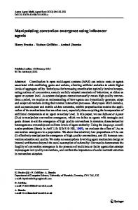
Fast Automatic Liver Segmentation Combining Learned Shape Priors with Observed Shape Deviation Marius Erdt, Sebastian Steger Fraunhofer IGD Cognitive Computing & Medical Imaging Darmstadt, 64283 Germany
[email protected] [email protected]
Abstract We present a novel statistical shape model approach for fully automatic CT liver segmentation. Unlike previous techniques, our method combines learned local shape priors with constraints that are directly derived from the current curvature of the model in order to restrict adaptation to regions where large deformations are expected and observed. Our approach is based on a multi-tiered framework that is more robust against model initialization errors than existing methods, because the model’s degrees of freedom are step-wise increased. We evaluated our method on a large data base of 86 CT liver scans from different vendors, protocols, varying resolution and contrast enhancement. For comparison, 50 of the scans were taken from 2 public data bases, one of it being the MICCAI’07 liver segmentation challenge data base. Evaluation shows state of the art results with an average mean surface distance between 1.3 mm and 1.85 mm compared to ground truth depending on the image resolution. With an average segmentation time of 45 seconds our approach outperforms other automatic methods.
1
Introduction
Fully automatic abdominal organ segmentation in Computed Tomography (CT) images plays an important role in medical imaging since it is a key enabler for many computer aided diagnosis applications. Robust automatic liver segmentation is still an unsolved problem, because shape and appearance of the liver may highly vary between scans due to different contrast phases, the presence of pathologies, variation in patient pose and breathing cycle and due to a per se high anatomical variation. We address these
Matthias Kirschner, Stefan Wesarg TU-Darmstadt Graphisch-Interaktive Systeme Darmstadt, 64283 Germany
[email protected] [email protected]
issues by a multi-tiered model based framework that constantly increases the model’s degrees of freedom (cf. section 3.3). As Ecabert et al. [3] do for the segmentation of the heart, we start the model evolution with an affine registration. We then perform classical statistical shape model (SSM) [1, 2] evolution and complete the segmentation with a two-step adaptation that combines SSM with local curvature constraints. We show that stepwise increasing the degrees of freedom significantly increases the initialization robustness (cf. section 4). SSMs are frequently used [5, 7, 13, 9, 8, 6] for liver segmentation because of their ability to constrain the segmentation to approximately match previously seen shapes of a training data base. However, segmenting only in the trained space is not sufficient to accurately match local regions of high curvature [9, 8, 6]. Therefore, SSM based methods usually add a (constrained) free-form deformation term to the optimization. Most of those terms constrain the shape globally [8, 6] which is usually not sufficient, since not all organ regions have the same amount of local variation. Similar to Kohlberger et al. [9], we use the local curvature learned from the training shapes to constrain the deformation of the model locally. However, we use an explicit shape representation [8, 6], because here local correspondence between the initial shape and the deformed shape during evolution is naturally given through landmarks. Since those learned shape constraints only reflect the expected local variation, we add a patient specific shape penalization (cf. section 3.1) which increases segmentation accuracy compared to methods using only learned shape (cf. section 4). An average surface dist. between 1.3 mm and 1.85 mm evaluated on a large test set of 86 CT scans of the liver including two challenging public data bases emphasizes the broad applicability of our method (cf. section 4). To our knowledge, no other liver segmentation approach was eval-
uated using such a large public data base. Starting with a limited number of degrees of freedom the average segmentation time could be limited to 45 sec. which outperforms other automatic methods.
2
Related Work
In the context of the liver segmentation competition held at a conference workshop of MICCAI 2007 [7], a data base of CT images was made publicly available in order to let teams compare their approaches. The majority of the best automatic methods use statistical shape knowledge [7]. Recent results show that both implicit [13] and explicit shape representations [8] are equally suited to segment the liver with high accuracy (1.37/1.02 mm mean error). Instead of using the 10 test cases for online competition, some teams are using the provided 20 training sets for evaluation [9, 12]. However, most methods are evaluated on a small amount of test cases (usually between 10 and 25 [13, 9, 8, 6, 12]). A test on a larger data base (174 scans) was performed in [10] with a reported 1.59 mm mean error after a manual removal of outliers (1.76 mm without outlier exclusion). However, a non-public data base from a single vendor was used for evaluation so it is unclear how the method would perform on the highly heterogeneous scans from the public competition data bases. It is also unclear how many high and low resolution scans were used. This is especially crucial since only the average surface distance was used as a metric for evaluation.
3
Locally Constrained Shape Model
Our SSM is built on 220 non-public reference shapes of the liver with N = 3612 corresponding landmarks using the approach of Cootes et al. [1]. In order to reduce the dimensionality of the model, axes with small variance are excluded. We choose the smallest dimension t such that P t i=1 λi captures 98% of the variance of the training data set, where λ1 ≥ . . . ≥ λ3N are the eigenvalues of the according covariance matrix C. The set of shapes modeled by the SSM are all shapes x ˆ in the form x ˆ =x ¯ + Eb, where E = (e1 | . . . |et ) is the matrix of retained eigenvectors and x ¯ is the geometric mean, i.e. the initial shape to be adapted to the image. The √parameters bi are restricted to be in √ shape the interval [−3 λi , 3 λi ] as used in [6].
3.1
Local Shape and Appearance Priors
Similar to [9, 4], we incorporate local shape variation into the deformation term. Since we use an explicit model, correspondence is given through landmarks. At
Figure 1. Trained local shape constraints define regions of differing elasticity (model after adaptation).
each point ti of all 220 training shapes the Gaussian curvature Cg (ti ) = κ1 κ2 is computed, where κ1 κ2 is the minimum and maximum principle curvature. Afterwards the mean curvature over all training shapes is stored as weight wi ∈ [0, 1] for every point pi of x ¯ to encode regions of different elasticity (Fig. 1). Some areas like the transition to heart, kidney and stomach potentially share only a fuzzy boundary with the liver. In order to prevent the model from leaking, we add a local gradient threshold ri to every model point pi and an adaptation weight vi which represents the influence of a found boundary point ai in the deformation (cf. section 3.3). Using 20 non-pathologic cases of the training base, for every point ti in each ground truth mesh the image gradient ∇g in the corresponding training image is computed. The threshold ri for model point pi is given by µi (∇g) − sdi (∇g), with µi (∇g) and sdi (∇g) being mean and standard deviation of the gradient at ti over the training set, respectively. vi ∈ [0, 1] is the current image gradient during deformation of pi mapped linearly to [µi (∇g) ± sdi (∇g)]. During adaptation, vi may be set to 0 by the boundary detection in order to deactivate the adaptation of points pi if no valid boundary point is found. This process is explained in the next section. Since a particular image may considerably deviate from trained samples, we derive image specific constraints directly from the current position of the shape model in the image. For every point pi of the model during deformation the current local Gaussian curvature ui ∈ [0, 1] is combined with the trained curvature wi and stored as δi = 1 − ((π/2 + arctan (β(wi + ui − s0 ))) α e−|(wi −ui )/σ| (wi /π)).
(1)
(a)
the model from leaking into neighboring structures. Image specific intensity constraints are calculated by first thresholding the image to L1 = [−50, 300]. The healthy tissue of all 86 test livers falls into that range. After examination of the intensity distribution of healthy liver tissue in ground truth segmentations, we conclude this distribution to be approximately Gaussian. Assuming there is a significant overlap of the model with the liver visible in the image, the histogram H of the model’s interior clamped to L1 contains a major peak representing liver tissue. Using H, we estimate a rough liver intensity range defined as L2 = [µH ± sdH ] with µH and sdH being mean and standard deviation of H, respectively. Both image specific shape and intensity constraints are updated in every iteration, i.e. with every deformation of the model.
3.2
(b)
Figure 2. (a) Weight function to combine trained local Gaussian curvature constraints w with observed local curvature u during adaptation. (b) Rule based boundary detection. A model point either gets a default boundary point D, a regular boundary point B or a deactivated boundary point N assigned depending on the search direction +/− and its state (inside/outside of estimated organ).
The weight function of eq. (1) is plotted in Fig. 2(a). It ensures that the resulting weight δi becomes 1 − wi if ui ≈ wi >> 0 and 1 otherwise. That means the adaptation is restricted to those regions which show a high curvature wi in the training and a similar high curvature ui in the model shape after adapting to the SSM space. We define high curvature as wi , ui > 0.4 and the similarity of ui and wi as ui − wi < 0.3. This results in the parameter settings s0 = 1.2 and σ = 0.2. In our tests these values yielded the best results and were used for evaluation. α and β control the smoothness of the function and are set to high values, e.g. 10 in order to clearly separate areas of high and low curvature. In contrast to using only trained constraints the described combination of trained and observed Gaussian curvature allows the model to better adapt to shapes not fully covered by the training space (Fig. 3) while at the same time prevents
Rule Based Boundary Detection
Standard SSM boundary detection is based on sampling local intensity patterns and the subsequent assignment of a fitness value to decide whether a point lies on the boundary or not [5, 7, 13, 9, 6, 15]. We enhance this scheme by a rule based system that deactivates boundary points in the adaptation in order to remove outliers. The remaining point positions are interpolated by the optimization. Fig. 2(b) shows the distinguished cases. A model point pi can either be in the state inside or outside (denoted as I and O in Fig. 2(b)) depending on whether Li = [µHi ± sdHi ] is ⊆ L2 , with Hi being the local histogram of an isotropically interpolated 9x9x9 neighborhood around pi . Samples along the point’s normal are then taken (−/+ denote the direction towards the model’s interior and exterior in Fig. 2(b)). If a point is outside, only search direction ’−’ is applied. If the fitness value is too small, but Li ⊆ L2 at all sample positions, a default boundary point at the end of the normal (5 mm) is set (D in Fig. 2(b)) in order to avoid that the model’s boundary stuck to local minima. If Li ⊆ L2 and the fitness value is sufficient, a boundary point (B in Fig. 2(b)) is assigned. The adaptation weight vi of an inside point is set to 0 if Li 6⊆ L2 . This case denotes a contradiction during the search, i.e. the state of pi is inside but something is found inside of the model that was not classified as organ tissue. Since we cannot decide whether this is a vessel/tumor or some organ foreign structure, the point is deactivated in the adaptation. We use the local gradient as fitness criteria and the weights r from section 3.1 as a fitness threshold. However, any other fitness criteria like the Mahalanobis distance between sampled profiles [2] could be used without changing rules. This makes our system simpler and more generic in comparison to other rule based boundary approaches [8].
3.3
Multi-Tiered Model Adaptation
Our initialization places the model axis-aligned below the right lower lung lobe. For automatic detection of the lobe we use simple voxel-counting operations similar to Kainmueller et al. [8]. Our multi-tiered adaptation pipeline then corrects translational errors and determines the correct orientation of the model as described in the following. After initialization, the model is adapted to the image by a four-step evolution. The degrees of freedom are accordingly increased in every step in order to allow a robust adaptation to shapes which differ a lot from the initial model in terms of position, orientation and local shape. In the first step, we allow only 12 degrees of freedom. That is, the affine transformation TA to register the found boundary points a described in section 3.2 with points p is determined minimizing P the current model 2 (T (p ) − a ) , with P being the set of point inA i i i∈P dices. This step is iteratively repeated until the sum of squared differences between corresponding points of two successive iterations do not differ significantly. The same stopping criteria will be used for the upcoming steps. The second step is a conventional SSM guided segmentation using the restricted shape parameters bi as defined before in order to approximate the real boundaries. The new model points S(p) are determined by S(p) = x ¯ + Eb.
Figure 3. Using local constraints, our multitiered model (dark outline) leaves the learned space (bright outline) without leaking into other neighboring structures.
Figure 4. Exemplary cases of the challenging IRCAD data base. Left: scan with 20 tumors inside of the liver. Right: a huge tumor at the lower liver lobe leads to a very uncommon liver shape. In such a case a precise segmentation of the liver is impossible if only trained shape priors are used.
(2)
The third step consists of step two coupled with the freeform deformation proposed by Ecabert et al. [3]. We constrain the free-form deformation by the local curvature and adaptation priors δi and vi defined in section 3.1. The new coordinates for p are calculated by minimizing E=
P
δi
P
2
((pi − pj ) − (S(pi ) − S(pj ))) 2 −vi (pi − ai ) , (3) with N (i) denoting the set of all neighbors of point pi . After convergence, the model already has a good alignment with the image. However, strong deviations from the trained space are still problematic. Some liver lobes are extremely long (cf. Fig. 3 left). The neighbor-distance-based regularization in equation (3) is too restrictive to let the model evolve in those regions. For the fourth step, we replace said regularization with the Laplacian differential mesh operator L(pi ) = pi − P 1 p j∈N (i) j , where #Ni denotes the number of neigh#Ni bors for point pi . This operator was proposed by Lipman et al. [11] for interactive mesh editing. L measures the deviation of a vertex from the centroid of its neighbors and thus preserves local detail properties of the surface. However, it is scale independent which allows a better local adaptation. i∈P
j∈N (i)
The new model coordinates are calculated by minimizing P 2 2 E = i∈P δi (L(pi ) − L(S(pi ))) − vi (pi − ai ) (4) After convergence of this last step, the segmentation is finished. Equations (3) and (4) form linear systems and can be solved very efficiently in a least squares sense.
4
Evaluation
We evaluated our approach using 4 non-overlapping sets consisting of 86 CT liver scans differing in resolution, contrast enhancement and present pathology. None of the test sets were used for training. Set MTEST is the test set of the MICCAI’07 liver challenge (10 scans), cf. [7]. Set MTRAIN is the training set of the same challenge (20 scans). We decided not to train our approach using this data, but instead
Table 1. Starting model deformation independently at the center of gravity of ground truth and at the automated calculated position results in the listed deviation of the final segmentation (cf. [7] for metrics). The first row shows the deviation for classical SSM adaptation, the second row shows the results for our multi-tiered approach. The results are averaged over 76 test scans. Method
Ovrl. Error Dev. [%] 1.02 0.23
SSM O UR APPROACH
Vol. Diff. Dev. [%] 1.31 0.15
Avg. Dist. Dev. [mm] 0.35 0.09
RMS Dist. Dev. [mm] 0.85 0.24
Max. Dist. Dev. [mm] 5.39 0.85
Table 2. Mean and standard deviation of volume and surface errors, cf. [7] for the 86 scans listed separately for each test set using the proposed fully automatic approach. Num. scans / test set 10/MTEST 20/MTRAIN 20/IRCAD 36/LOWRES
Ovrl. Error [%] ±SD 8.62 ±1.49 7.54 ±1.18 10.34 ±3.11 12.35 ±1.98
Vol. Diff. [%] ±SD 1.32 ±2.04 1.28 ±2.15 1.55 ±6.49 -4.53 ±4.05
Figure 5. From left to right: qualitative segmentation results for test sets MTRAIN, IRCAD and LOWRES. Each column shows transversal (top), sagittal (middle) and coronal (bottom) view.
Avg. Dist. [mm] ±SD 1.54 ±0.44 1.30 ±0.33 1.74 ±0.59 1.85 ±0.34
RMS Dist. [mm] ±SD 3.13 ±0.99 2.67 ±0.97 3.51 ±1.16 3.27 ±0.68
Max. Dist. [mm] ±SD 25.90 ±7.28 26.52 ±10.07 26.83 ±8.87 23.09 ±5.62
Chall. Score 68.41 71.33 61.67 60.43
to use it as an additional test set. We do this in order to compare our method to other approaches which use this set for evaluation [9, 12]. In order to add very challenging data sets to the evaluation we use the public 3D-IRCAD data base (www.ircad.fr) built for comparison of segmentation algorithms (test set IRCAD). 75% of the 20 provided scans (axial spacing between 1 and 4 mm) having hepatic tumors, which makes a robust segmentation extremely difficult (cf. Fig. 4). Since most algorithms are only tested on highresolution data we add a set LOWRES which consists of 36 thorax/abdomen scans from a Siemens Sensation scanner with the standard slice spacing for abdominal control scans of 5 mm. All 86 scans are taken to evaluate the overall segmentation accuracy using the MICCAI’07 challenge metrics [7]. For evaluating the initialization robustness, MTEST is excluded since the ground truth is only available to the challenge initiators. We evaluated the model initialization accuracy taking the center of gravity of the ground truth segmentation as reference [14]. Mean and standard deviation are 35 ± 14 mm for MTRAIN, 40 ± 13 mm for IRCAD and 44 ± 17 mm for LOWRES. However, the effect of this error can be corrected by our method as Table 1 shows. The avg. mean surface distance of the final segmentation deviates only by 0.1 mm using ground truth or automatic model positioning. In contrast, classical SSM segmentation shows higher dependency of initial positioning (Table 1). The final segmentation results are listed in Table 2 and shown in Fig. 5 for exemplary scans of the test sets. MTEST was submitted to the organizers of the challenge. Fig. 3 shows that our combination of trained shape constraints with ob-
served shape deviation allows the model to robustly leave the trained space without leaking into neighboring structures. The fully automatic segmentation of one case takes in average 45 seconds on a 2.93 GHz Quad Core CPU.
5
Discussion and Conclusion
We have presented a novel fully automatic multi-tiered statistical shape model for the liver that combines learned local shape constraints with observed shape deviation during adaptation. Said combination allows the model to leave the trained space without leaking into neighboring structures. In comparison with using only trained local curvature constraints [9] our method yields significantly superior results (71.3 to 66.7 score). With a mean surface distance of 1.3 to 1.54 mm for the commonly used [7] evaluation sets MTRAIN and MTEST our approach places among the top automatic methods [7, 13, 9, 8, 6, 10]. However, in contrast to other methods [7, 13, 8, 6] (10 test scans), we evaluated our approach using a large heterogeneous test set of 86 scans. Adequate comparability between methods is only possible if evaluation is performed on publicly available test cases. Therefore, we included the 3D-IRCAD data base (www.ircad.fr). We decided to use this data base since it is a very challenging data base for segmentation. Some scans contain up to 46 tumors (Fig. 4 left), some of them being extremely large (Fig. 4 right). Nevertheless our approach is able to segment this set with a very high accuracy. Because most methods [7, 13, 9, 8, 6] are mainly tested on highresolution data we evaluated our approach using 36 scans with the standard slice spacing for abdominal control scans of 5 mm. Our approach is also able to segment this data with a high accuracy which emphasizes the broad applicability of our method. Unlike other methods [7, 13, 9, 8, 6, 10], we evaluated the effect of model initialization on the final segmentation and showed that our method is more robust against model positioning than standard SSM segmentation. The mean surface error of the final segmentation deviates in average only by 0.1 mm between ground truth positioning and a coarse automatic initialization. The adaptation in our multi-tiered pipeline is split into single steps starting with a limited number of degrees of freedom. This significantly increases the overall convergence speed of the adaptation to an average of 45 sec. which outperforms other automatic methods [8, 6, 13] (3-15min.). In future work, we plan to combine our rule based boundary detection with an appearance model for tumors in order to increase the performance especially for cases with prominent pathologies.
References [1] T. Cootes, C. Taylor, D. Cooper, and J. Graham. Active shape models - their training and application. Computer Vi-
sion and Image Understanding, 61(1):38–59, 1995. [2] R. Davies, C. Twining, and C. Taylor. Statistical Models of Shape - Optimization and Evaluation. Springer Verlag, 2008. [3] O. Ecabert, J. Peters, H. Schramm, C. Lorenz, J. von Berg, M. J. Walker, M. Vembar, M. E. Olszewski, K. Subramanyan, G. Lavi, and J. Weese. Automatic model-based segmentation of the heart in ct images. IEEE Trans. Med. Imaging, 27(9):1189–1201, 2008. [4] M. Erdt and G. Sakas. Computer aided segmentation of kidneys using locally shape constrained deformable models on ct images. In SPIE Medical Imaging 2010, pages 762419– 762419–8, 2010. [5] T. Heimann and H. Meinzer. Statistical shape models for 3d medical image segmentation: A review. Medical Image Analysis, 13(4):543–563, 2009. [6] T. Heimann, H. Meinzer, and I. Wolf. A statistical deformable model for the segmentation of liver ct volumes. In MICCAI 2007 Workshop Proceedings: 3D Segmentation in the Clinic: A Grand Challenge, pages 161–166, 2007. [7] T. Heimann, B. van Ginneken, M. Styner, and et al. Comparison and Evaluation of Methods for Liver Segmentation from CT datasets. IEEE Trans. Med. Imaging, 28(8):1251– 1265, 2009. [8] D. Kainm¨uller, T. Lange, and H. Lamecker. Shape constrained automatic segmentation of the liver based on a heuristic intensity model. Proc. MICCAI Workshop 3D Segmentation in the Clinic: A Grand Challenge, pages 109– 116, 2007. [9] T. Kohlberger, M. G. Uzunbas, C. V. Alvino, T. Kadir, D. O. Slosman, and G. Funka-Lea. Organ segmentation with level sets using local shape and appearance priors. In Proc. MICCAI 09, pages 34–42, 2009. [10] H. Ling, S. Zhou, Y. Zheng, B. Georgescu, M. Suehling, and D. Comaniciu. Hierarchical, learning-based automatic liver segmentation. In CVPR08, pages 1–8, 2008. [11] Y. Lipman, O. Sorkine, D. Cohen-Or, D. Levin, C. R¨ossl, and H.-P. Seidel. Differential coordinates for interactive mesh editing. In Proceedings of Shape Modeling International, pages 181–190. IEEE Computer Society Press, 2004. [12] Y. Song, A. J. Bulpitt, and K. W. Brodlie. Liver segmentation using automatically defined patient specific b-spline surface models. In Proc. MICCAI 09, pages 43–50, 2009. [13] A. Wimmer, G. Soza, and J. Hornegger. A Generic Probabilistic Active Shape Model for Organ Segmentation. In G.-Z. Yang, D. Hawkes, D. Rueckert, A. Noble, and C. Taylor, editors, Proc. MICCAI 09, volume 5762, pages 26–33, Berlin Heidelberg, 2009. [14] J. Yao and R. M. Summers. Statistical location model for abdominal organ localization. In Proc. MICCAI 09, pages 9–17, 2009. [15] Y. Zhen, A. Barbu, B. Georgescu, M. Scheuering, and D. Comaniciu. Fast automatic heart chamber segmentation from 3d ct data using marginal space learning and steerable features. In 11th Int. Conf. on Computer Vision (ICCV), pages 1–8, 2007.