Schedae Informaticae Vol. 24 (2015): 159–177 doi: 10.4467/20838476SI.15.015.3997
Evolutionary Algorithm for Particle Trajectory Reconstruction within Inhomogeneous Magnetic Field in the NA61/SHINE Experiment at CERN SPS
´ ski1,2 Oskar Wyszyn 1
Faculty of Physics, Astronomy and Applied Computer Science Jagiellonian University, Lojasiewicza 11, 30-348 Krak´ ow, Poland 2 CERN, CH-1211 Geneva 23, Switzerland e-mail:
[email protected]
Abstract. In this paper, a novel probabilistic tracking method is proposed. It combines two competing models: (i) a discriminative one for background classification; and (ii) a generative one as a track model. The model competition, along with a combinatorial data association, shows good signal and background noise separation. Furthermore, a stochastic and derivative-free method is used for parameter optimization by means of the Covariance Matrix Adaptation Evolutionary Strategy (CMA-ES). Finally, the applicability and performance of the particle trajectories reconstruction are shown. The algorithm is developed for NA61/SHINE data reconstruction purpose and therefore the method was tested on simulation data of the NA61/SHINE experiment. Keywords: tracking, event, reconstruction, particle, high, energy, physics, HEP, NA61, SHINE, CERN, TPC, magnetic, field, CMA, evolutionary, strategy, bayes, generative, discriminative.
1.
Introduction
In the field of High Energy Physics (HEP), reconstruction of charged particle trajectories is a challenging task in terms of efficiency and computational complexity. The first commonly used techniques were histogramming and Hough transformation [1]. Unfortunately, histogramming shows poor efficiency, when dealing with high density of tracks and relatively high measurement uncertainty, whereas the Hough Transformation is characterized by high computational complexity compared to its efficiency.
160 The flaws of employed methods became more visible during the quest for scientific discoveries which lead to higher energies, implying higher multiplicity of particles. In late 90’s the Kalman filter was introduced to event1 reconstruction in HEP by Billoir [2–4] and Fruhwirth [5], becoming the most popular algorithm for particle trajectory reconstruction. The Kalman filter [6] lies under most of track reconstruction algorithms used in modern experiments, including experiments located at the Large Hadron Collider (LHC) [7]. The LHC, located at CERN in Geneva, is the world’s largest and most powerful particle accelerator. All four LHC experiments based their algorithms on the Kalman filter with great success: ATLAS [8, 9], CMS [10–12], ALICE [13, 14] and LHCb [15–17]. Despite of the success of Kalman filter, there are parallel efforts to develop new tracking algorithms which use much simpler models, and at the same time provide similar performance without using an approximation. Often, creation of the state transition, control and observation matrices is difficult, especially when dealing with multidimensional data. Furthermore, a desired feature is to eliminate slow combinatorial algorithms for newly included particle detectors in the system. In order to simplify such excessive processes, a search for a more general algorithm was performed. The field of Machine Learning turned out to be a natural choice. For reference, many techniques were studied, namely the Cellular Automaton for the LHCb Outer Tracker [18] as well as a recursive neural network known as Hopfield Network in the LHCb Muon System [19], developed in the LHCb experiment. Another experiment, ALICE, presents an applicability of the Denby-Peterson network for the Inner Tracking System [20–22]. Those new methods are often accompanied by the Kalman Filter[18, 20–22]. Applying a search for potential points for extension of track candidates, these methods preserve the drawback of Kalman filter. A detailed overview of the state of event reconstruction techniques in HEP is provided in [23] and [1]. In this paper, a novel evolutionary algorithm is presented along with application on particle trajectory reconstruction in the NA61/SHINE experiment, located at the CERN SPS accelerator. The facility of NA61/SHINE experiment [24] consists of many sub-detectors, where the key componets are the Time Projection Chambers (TPC) [25] shown in Fig. 1. Vertex TPCs are considered problematic due to the presence of the magnetic field and very high track densities. Therefore, our study is focused on the vertex TPC local track reconstruction.
2.
The raw data
In order to understand the algorithm, the mechanism of acquiring the data has to be presented. First, we will describe detector working principles and the raw data output. Second, the clusterization algorithm will be explained, which is the last processing 1 An event refers to the results of a single fundamental interaction, which took place between subatomic particles.
161
Superconductive Magnets
BEAM
Main TPC Left
Vertex TPC 2
Vertex TPC 1 Target
Gap TPC
Main TPC Right
Particle Trajectories
Figure 1. Simplified detector configuration of the NA61/SHINE facility. The beam, consisting of particles accelerated to relativistic speeds, is projected on a fixed target. The produced particles traverse the Time Projection Chambers (TPCs), where their trajectories are bent by the ∼ 1.5T magnetic field of the superconducting spectrometer magnets. step before tracking. Finally, the nature of the particle trajectories is briefly described in order to define the problem which needs to be solved by the presented algorithm.
2.1.
Time Projection Chambers
A Time Projection Chamber (TPC), indicated in Figure 1, consists of particle detectors placed inside a volume of noble gas located in a homogeneous electric field. A particle passing within the TPC sensitive volume ionizes the gas. The resulting primary ionization electrons drift toward the amplification-and-readout plane due to the electric field, as show in Figure 2. The amplification-and-readout plane, containing an array of readout pads equipped with an amplifier, a time sampler and charge digitizer electronics, provides the digital data about the ionization trace. The Z coordinate along the track is parameterized by the padrow location index. At a given padrow, the X value and Y value are derived from the charge deposit profile of the track intersection with the padrow: the X coordinate is determined by the charge deposition intensity along pad index, whereas the Y coordinate (drift depth) is determined from the charge deposition profile in terms of time slice index, after Detector/clusterization. The described structure of raw data is shown in Figure 3. A number of detector effects can slightly influence the shape of a measured charge deposition cluster of a track intersection with a padrow. For instance, particles traversing the bottom part of the detector, and thus having a larger drift path, produce clusters with a larger radius due to charge cloud diffusion in the working gas. This implies a deterministic distortion effect on the signal. Fluctuations of the ionization process along with the electronic
162
x
y
Time slice
z
Elecric field Padrow
Track
Electrons
Detection volume
Figure 2. Simplified illustration of TPC working principle.
pickup noise on the readout pads, on the other hand, superimpose a statistical uncertainty on the measured charge depositions. The ensemble of all such detector effects complicates the task of track pattern recognition in the system. Further readings on the data readout is provided by [26] and [27].
2.2.
Clusterization of ADC signals on a padrow
The number of deposited charge ADC signals within one event amounts to about 5 × 10⁷ regardless what type of reaction is considered. It is a considerable amount of data, especially in a situation where millions of events per reaction are collected. Therefore, reduction of the data is needed by means of charge clusterization on each padrow. This approach leads to significant reduction of the data size (factor of around thousand for low particle multiplicity events). We aimed at having a fast clusterization and therefore used a simple algorithm with value based start and stop criteria and subsequent quality assessment of parameters such as shape, maximum and average values of ADC signals. In the end, we produce the clusters with a point in the 3D space as the main attribute.
163
250
160
Signal
Pad
VTPC1, Sector 2 180
200
140 120
150 100 80
100
60 40
50
20 2
4
6
8 10 12 14 16 18 20 22 24
0
Row
Figure 3. Maximal value of digitalized charge within one time slice (ADC signal) measured for every pad in second sector of vertex TPC 1. One can recognize trajectories produced by four traversing particles.
2.3.
Particle motion
Recognition of particle trajectories in chambers without presence of magnetic field such as MTPCs, reduces the problem to finding straight lines. However, when magnetic field is applied, the equation of motion has to incorporate the deflection caused by the Lorentz force Fl Fl =
dp = q · (E + v × B) ≈ q · v × B dt
(1)
In case of NA61/SHINE, the strength of the electric field in the TPCs is of the order of ∼ 20kV /m, whereas the magnetic field force is approximately ∼ 3 · 108 V /m. Therefore, the neglection of electric field is justified. The elapsed time t along the track flight can be reparameterized using flight path length s as dt = ds/v, where v = |v| is the magnitude of velocity vector. Introducing p = |p| for the momentum magnitude, the unit vector e = v/v = p/p gives us the following equation de =
q · e × B · ds p
(2)
Afterwards, using a simple but tedious mathematical transformation, the path length s is reparameterized by detector coordinate z, see for instance [28]. This leads to a system of differential equations, z being the running parameter, resulting in the following extrapolation operator
164 Q : T × R → T,
(3)
where T is a track parameters vector space. Thus, an outcome of the Q, given a track parameter vector Θ0 and destination z, is equal to ˆ = Q(Θ0 , z). Θ
(4)
Often instead of the above equation, an approximation is used, e.g. a helix track. That is only possible in situations where the magnetic field is relatively homogeneous. However, to acquire a homogeneous magnetic field in practice is a challenging task, and therefore the helix equation may not always be a good approximation to the true solution of our differential equation. Nevertheless, the helix approximation may be handy for rough track parametrization in the parts of an algorithm where great accuracy is not required.
3.
Evolutionary tracker
TimeSlices
The evolutionary tracker is a recursive algorithm that uses a series of measurements obPadrow served over an elapsing parameter such as 250 time or z coordinate in our case, and pro225 duces estimates of a track parameters Θ. 200 Value 250 The algorithm involves two stages: predic175 tion and measurement update. A prediction 200 150 is made by extrapolating a track parameter 150 125 vector with equation (3) to a Z position of 100 100 a next measurement, namely a cluster as in 50 75 Section 2.2. 0 50 The proposed algorithm consists of three principal components. (i) Model of an event 25 – a whole event is modeled using a discrim0 0 25 50 75 100 125 150 175 inative model of a background and a generPads ative model of a particle trajectory. CompeFigure 4. Values of digitized charge tition between those models shows good sigfor every pad and every time slice nal to noise separation. (ii) Measurementfor an example padrow. The clusters to-track association – this is performed us(circular spots), determine locations ing breadth search along with sorting of the where particles traversed the particu- measurement in order to construct time-line. lar padrow. (iii) Continuous track parameter optimization – is realized by means of the Covariance Matrix Adaptation Evolutionary Strategy (CMA-ES), stochastic and derivative-free method proved to be working for an objective ill-conditioned function with discontinuities where other derivative based and Quasi-Newton methods failed. In this section each of the components are described.
165 3.1.
Model of an event
The event model consists of the two competing models, the generative model of a track and discriminative model of a background. The aim of the competition is an efficient method to separate signal from noise. In this section both models are described along with a reason why the generative model was used for a track, whereas discriminative models shows, in general, better performance [29]. A prior probability is estimated from simulated training samples and a likelihood function is constructed based on known detector resolution. A one variable logistic regression was used for the background, which proved to be sufficient.
3.1.1.
Na¨ıve Bayes trajectory model
The Na¨ıve Bayes trajectory model assumes all parameters to be independent and identically distributed as the track parameters are. Interestingly, the Na¨ıve Bayes demonstrates good performance in practice [30], also for problems which violate the assumption of statistical independence. The explanation of this phenomenon can be found in [31], which shows that the optimality of Na¨ıve Bayes approach does not depend on the independence attribute and the applicability is much greater than the original restrictive assumptions would suggest. The main reason of choosing a generative model is the fact that uncertainty of track cluster position estimates are well known, hence there is no need to estimate it from scarce labeled data. With constant arbitrary likelihood parameters, only a prior probability estimate is required. Therefore, the Na¨ıve Bayes model was chosen although the the logistic regression is expected to overtake the performance of the Na¨ıve Bayes method as the number of training samples is increased [29]. The particle trajectory model is described as Posterior probability
z }| { ˆ P (Θ|S(c))
Likelihood
∝
ˆ P (Θ) | {z }
Prior probability
z }| { ˆ P (S(c)|Θ)
(5)
where c = (x, y, z, s1 , . . . , sn ) stands for a cluster with center of gravity located at (x, y, z) along with charge deposition ADC signals (s1 , . . . , sn ) in the cluster. The ˆ denotes an estimation for a track parameter vector Θ = p ⊕ o, where symbol Θ p = (px , py , pz ) denotes the particle momentum vector at a starting point o = (x, y, z) and ⊕ denotes concatenation operator (dim(Θ) = dim(p) + dim(o)). The operator S : T ∪C → R3 produces a three dimensional Euclidean space vector S(ξ) = (ξx , ξy , ξz )
(6)
where C is a cluster parameter vector space. The model (5) consists of two components: likelihood function of a cluster, given a track; and an a priori probability of a particular track parameter vector. The likelihood is defined in the following manner: ˆ = P (S(c)|Θ, ˆ Σ) ∼ N (Θ, ˆ Σ) P (S(c)|Θ)
(7)
166 ˆ is an estimate of parameters Θ being where ‘∼’ denotes equality in distribution, Θ ˆ z and Σ is a diagonal covariance extrapolated by equation (3) to a position cz = Θ matrix. The parameters of the likelihood function are contained in the diagonal covariance matrix Σ = diag{σx2 , σy2 , σz2 } (8) Note that the value of σz2 is irrelevant as z position of a cluster is not a stochastic variable, but is determined by the padrow location. The prior probability is an empirical distribution estimated from simulated data (see Section 4.1.) using a maximum likelihood estimator. The data binning technique along with the Gaussian Kernel smoother is used in order to reduce the memory footprint of the probability density function (PDF), so that the size remains constant regardless the amount of samples that have been used. The empirical prior probability was chosen instead of a conjugate prior, as the distribution may change significantly in a way that one distribution cannot describe all possible priors. The fact, that the training data are simulated provided an opportunity for a wide range of studies, such as selection of desired particle charge or tracks with desired pseudo-rapidity2 . The Bayesian approach makes it possible to consider some patterns more likely over others, and opens new possibilities for new techniques in physics analysis.
3.1.2.
Logistic regression as a background model
Background noise
1.0
Probability
0.8
0.6
0.4
0.2
0.0
0
50
100
150
ADC value
200
250
Figure 5. Scaled probability mass distribution of background noise PN , using maximum ADC feature value of a cluster.
On the other side of the competition, the discriminative model is used to describe the background. It is a simple onedimensional model which uses only one single feature of clusters, namely maximal value of ADC signal within a cluster. For this purpose, labeled real data has been used. The probability mass distribution can be observed on Figure 5. Note that cluster with maximum ADC equals 255 is very likely to be a noise as it indicates a saturation in the electronics. Therefore, the final posterior probability is given by P (Ω|c) = PN (max(R(c))),
(9)
with operator from cluster to ADC signal vector space R : C → A R(c) = (cs1 , . . . , csn )
(10)
2 Pseudo-rapidity is a commonly used spatial coordinate, describing the angle of a particle relative to the beam axis.
167 which returns a vector of a n ADC signals of a cluster of dimension n. The Ω denotes a background class and PN is the probability mass distribution of maximum ADC value of a noise cluster. Despite of its simplicity, this noise model is seen to work quite well as a competitor to track model. It prevents attaching a cluster to a track is that does not very likely belong to any track because of its unlikely signal amplitude and therefore it reduces the number of outlier clusters on track candidates. In order to avoid overtraining, the Kolmogorov-Smirnov test is used on consecutive distribution updates until it reaches the significance level of α = 0.001.
3.2.
Measurement-to-track association
In this section a competition algorithm is described along with a decision rule, which is used in order to assign a cluster to a particular track or to background. An important issue in tracking algorithms is a way to determine number of objects as well as how to reach good computational efficiency of data association. The computational efficiency has been accomplished using a greedy algorithm on reduced search space, using a searching cone. Because of that, global optimum is not guaranteed, however it provides good performance, as presented in a later section. Although all measurements are available at the same time, the algorithm proceeds using clusters ordered along the z coordinate which can be treated as a running time. To be precise, it processes the clusters in opposite directions to natural time elapse, namely towards the target. This approach is justified by the fact that the density of tracks drops along the detectors in the downstream direction, and therefore we start from the regions of smallest density. The reason of the lower particle trajectory density in the downstream region is the initial opening angles between tracks, accompanied by the spreading effect by the magnetic field. The decision rule is defined in the following manner ( ϑ, if p(c) ≥ 1 δ(c) = (11) Ω, otherwise with the posterior probability ratio arg max P (ϑ|c) p(c) =
ϑ∈T
P (Ω|c)
(12)
where T denotes a set of track parameter vectors. The δ(c) function governs measurement association to a particular track/seed or to background. The latter implies a new track creation as the background cluster may belong to an other, yet undiscovered track. The initial step of track creation is called seeding: a new track object without estimated parameters is called a seed. During this stage, the seed collects all clusters within the search cone which do not belong to a track, but may share the cluster with other seeds. The overall mechanism of track competition is illustrated on Fig. 6.
168 As we follow the particles of interest in the detector in the upstream direction, it is possible to design a cone which will reduce the measurement search space. Therefore, a cone is defined which is governed by the following inequalities q (cnx − cx )2 + (cny − cy )2 (13) tg(β) ≥ |cnz − cz | and d ≥ |cnz − cz |
(14)
where β is a cone generatrix angle, cn is a last (with highest z value) measurement of a track and d is a maximum acceptable gap within a track. Collected clusters within the cone can be seen as a tree as illustrated in Fig. 7. The breadth search along with a prior probability function is used to find the most likely branch of the tree, that is to become a new track with the parameters estimated using the clusters solely from this branch. The remaining clusters are then released. The seed becomes a track candidate when the estimate of its parameters becomes possible, namely, when the following equation is satisfied h ≥ dim(p) (15) where h denotes level of a seed tree. Otherwise, direct comparison of tracks is not possible. Therefore, as mention above, the seed may accept and share all clusters which were not associated with a track. In case when (13) is satisfied, the track parameter vector is estimated for a path from a leaf (the newest cluster) until the tree root. When the parameters are estimated, the posterior probability is calculated and stored for every possible parent. Afterwards the estimated parameters from the most probable branch is chosen. A detailed data association algorithm is provided in the form of pseudo-code (Alg. 1). In the end, a second iteration over clusters is performed for reassociation of clusters improperly classified to the background using tracks found in a previous trial. In this stage, new tracks are not created.
3.3.
Continuous parameters optimization
Association (see Section 3.2.) of a new cluster naturally provides additional information, so a better trajectory estimate can be achieved. Therefore, every new assignment yields parameter optimization as shown at line 10 of Algorithm 1. In order to produce a new estimate of Θ the CMA-ES [32,33] algorithm has been chosen. It is a stochastic and derivative-free evolutionary algorithm which allows the method to work whereas Quasi-Newton methods fail. The chosen approach is regarded to be robust for a nonconvex functions which can comprise discontinuities, spikes or being ill-conditioned. Thus, the CMA-ES [32] in particularly is useful for solving ‘black box’ scenarios, where the knowledge about the underlying function is limited or an algorithm should not depend on that knowledge. The latter feature is very useful when the objective function significantly changes: severe modification to the algorithm is not needed, because of this property.
169 Figure 6. Illustration of the data association decisions made in a typical situation. The window slides from the left (downstream) to the right (upstream) pad-row by pad-row. 1) Failed to find a suitable track, thus a new seed is created before classification as a background; 2) P (Ω|c) < P (Θ|c). It is not the most probable candidate. It will become a new seed and later classified as a background; 3) P (Ω|c) > P (Θ|c), therefore being background is more likely, nevertheless it gets a chance as a seed, to form a track. In the end it will become a track Φ; 4) Looks for the most probable parent between Φ and Θ; 5) Being background wins, so a seed is created and it will be transformed to a track Γ.
Figure 7. Illustration of the breadth search performed on a seed (within the gray cone). 1) The root of a seed tree; 2) P (Ω|c) < P (Θ|c). It is not the most suitable candidate. Furthermore it will not became a seed; 3) P (Ω|c) > P (Θ|c). Classified as a background, nevertheless it becomes as a seed first; 4) Good track cluster. 5) The track is formed, thus a breath search is not performed. A new cluster is attached to the track.
The CMA-ES consists of three main steps: (i) offspring generation – new solutions (offspring) are generated by sampling a multivariate normal distribution; (ii) selection and recombination – for each offspring an objective function is evaluated; (iii) adapting a covariance matrix and a mean; see [34] for more detailed introduction. For the algorightm to work, only an objective function f : Rn → R is required to be defined.
170
Algorithm 1 Probabilistic data association 1: 2: 3: 4: 5: 6: 7: 8: 9: 10: 11: 12:
procedure PDA(cluster) for all tracks do . Including mature seeds probabilities[track] ← P (track | cluster) end for bestT rack ← Max(probabilities) if probabilities[bestT rack]