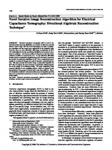
Figure 5. Sample slices of a breast tomosynthesis image: (a) z = 0.1 cm, (b) z = 1.5 cm, (c) z = 3.6 cm. 0. 0.02. 0.04. 0.06. 0.08. 0.1. 0.12. 0.14. Y. 0.05 Z. 0.02 0.04 ...
Nonlinear image reconstruction algorithm for diffuse optical tomography using iterative block solver and automatic mesh generation from tomosynthesis images Qianqian Fanga , David Boasa , Greg Bovermanb , Quan Zhanga , Tina Kauffmana a Massachusetts
General Hospital, Charlestown, MA 02148 USA. University, Boston, MA 02115 USA.
b Northeastern
ABSTRACT In this paper, we report a nonlinear 3D image reconstruction algorithm featuring 3D finite element forward modeling with an iterative multi-right-hand-side solver and an automatic mesh generation technique for efficient geometry modeling. The forward mesh was generated based on 3D tomosynthesis images acquired simultaneously with optical measurements. An efficient iterative solver based on a QMR algorithm with the capacity of solving multi-RHS was used to enhance the computational efficiency. The mesh generation algorithm was developed based on a moving mesh process and is able to generate high-quality mesh with low computational complexity. In addition, an approximated adjoint method was used to form the Jacobian matrix for the inverse problem. The performance of the was satisfactory performances in numerical simulations. For a typical reconstruction, the run-time was under 5 minutes on a Pentium-based PC. It is worth mentioning that the mesh generation module not only works for binary 2D or 3D image stacks, but also for any other binary description of the object, which makes it generalizable to many other potential applications. Keywords: Breast Imaging, Diffuse Optical Tomography, Mesh Generation, Tomosynthesis
1. INTRODUCTION Diffuse optical imaging has received increasing attention in the past decade for various clinical applications [1– 3]. The distinct absorption spectra of oxygenated and de-oxygenated hemoglobin in the near-infrared (NIR) range give diffuse optical imaging the unique capability to detect hemodynamics and the associated metabolism non-invasively. This functional information is practically valuable in cancer studies because tumors usually demonstrate abnormal vasculature structures and metabolism rates compared with normal tissues. The dozens of the research and commercial diffuse optical imaging systems developed across the world generally can be categorized as either spectroscopic systems and tomographical systems (or DOT). The former usually refers to the use of multi-spectral illumination to recover functional responses at limited measurement sites. In many cases, spectroscopic systems focus on pinpointing pathological assessment at pre-selected locations. NIR light with either discrete frequencies or a continuous spectrum can be found in these systems. In contrast, tomographical systems utilize spatially distributed source/detector arrays and aim at probing internal tissue structures or dynamics. To improve measurement efficiency, various signal-encoding techniques, such as frequency-encoding and time-multiplexing schemes, are frequently used in tomographical systems. Very often, in order to obtain functional information, illumination of multiple wavelengths is also required, which blurs the boundaries between spectroscopic and tomographical systems. Despite the unique feature it possesses, diffuse optical imaging usually suffers from low resolution and specificity. To remedy this, various approaches were investigated, including, injecting fluorophores to enhance the specificity or using other modalities as spatial prior to improve resolution have drawn significant attentions. The second approach has led to the development of many enhanced diffuse optical imaging systems such as MR-guided optical breast imaging systems [4] and the X-ray-guided DOT system discussed in this paper. At Massachusetts General Hospital (MGH) Martinos Imaging Center, we have developed a diffuse optical tomographical system primarily for breast cancer detection [5]. This system can be used stand-alone or in conjunction with conventional 2D mammography, or even with 3D tomosynthesis systems, to produce co-registered X-ray/optical images. Mammography is currently the most popular choice for regular breast screening in the
US. The cost of mammography equipment is relatively low compared that of MR-based breast imaging systems; the same is true for the patient’s cost for scanning. Unfortunately, the X-ray contrast in mammography images provides mostly morphological information and cannot tell the functional status of the tissue. This makes it difficult for doctors to find tumors or to determine the malignancy of the abnormalities. With the combined X-ray/optical imaging, we can provide both the morphological and pathological information simultaneously, which might help clinical practitioners in breast cancer assessment or monitoring during tumor treatment. The optical measurements are reconstructed with the Gauss-Newton method to recover the internal optical and functional information. In the reconstruction, the scattered light distribution inside tissues is modelled with the finite-element method (FEM) where the mesh was generated from the mammography scans if presented. The conventional approach for mesh generation from 2D or 3D medical images typically involves the following steps: 1) a segmentation or thresholding process; 2) segment surface extraction and smoothing; 3) mesh generation based on advancing front algorithm or other methods; 4) mesh optimization or “jiggling.” The process is technically complicated and not easily performed by researchers without training in mesh generation. Moreover, the computational complexity is high and the quality of the generated mesh is not ensured. In 2004, Persson and Strang [6] proposed a high-quality mesh generation algorithm based on physical equilibrium and a distancefunction description of geometries. This algorithm is conceptually straightforward and exceptionally simple in implementation. However, when the geometries become complicated, the distance function description becomes inefficient and the computational overhead becomes significant, not to mention that it is impossible to represent many geometries, for example, the segmented regions from medical images, by distance functions. Based upon the distance-function algorithm, we proposed an improved mesh generation algorithm using a more convenient binary-function description of geometries along with several other improvements. In this paper, we first give a brief overview of our imaging system hardware (Section 2.1). Then we focus on the image reconstruction process, especially the mesh generation algorithm from binary geometries (Section 2.2) and the performance of a multi-RHS iterative solver (Section 2.4). The forward FEM equations, the adjoint method in building Jacobian matrix and the Gauss-Newton update equations are also mentioned, in Section 2.3. Numerical examples including reconstructions of simulated and measured data are reported in the Results section. We conclude the paper by summarizing the findings as well as problems we perceived in the implementations.
2. METHODS 2.1. Instrument Overview The imaging system built at the MGH Martinos Imaging Center is called TOBI (tomographical optical breast imaging). This system includes a radio-frequency (RF) modulated imaging subsystem and a continuous-wave (CW) imaging subsystem. The TOBI optical probes was designed to mount and fit in GE-based 2D mammography and 3D tomosynthesis machines. The probes work in a transmission mode with sources and detectors on opposite sides of the compressed breast. The source and detector fibers on the probes were mapped into three groups corresponding to the three standard mammography views, i.e., Cranio-Caudal View (CC), Left Mediolateral Oblique View (LMLO) and Right Mediolateral Oblique View (RMLO) [7]. The fibers of each group are connected to a quick connector. This design allows us to switch the scanning area conveniently according to the doctor’s preference in clinical examinations. The CW subsystem can be further divided into a frequency-encoded CW imager, referred to as CW5 (TechEn, MA), and an optical multiplexer, referred to as the MUX (Innovations in Optics, MA). CW5 provides 32 sources (of which half are 780nm lasers and the other half are 830nm lasers) and 32 detectors. These lasers are encoded around the central frequency 9.0kHz with 200Hz spacing. The MUX unit has 6 lasers with wavelengths ranging from 690nm to 980nm. All MUX lasers are mixed and fast-switched to 150 locations on the source probe by a computer-controlled Galvometer. The dowelling time for each location is about 20 milliseconds. The use of MUX greatly enhanced the dynamic range of the signal and improved the spatial coverage of the measurement. In comparison, the RF imager is less sophisticated, consisting of 40 sources and 8 detectors. Similar to the MUX, a sequential scheme is used for RF sources where an optical switch is used to multiplex between 40 locations and two lasers, 780nm and 830nm. The RF measurement are used to decouple the absorption from scattering and provide coarse spatial information of the breast heterogeneities; the MUX and the CW5 measurements, on the other hand, target at higher resolution and refined image on top of or simultaneously to RF data reconstruction.
In clinical experiments, the source and detector probes are mounted and locked into a radio-translucent cassette on top of the mammography compression table. By choosing the appropriate scanning view (i.e., CC, LMLO or RMLO), the patient’s breast is positioned between the probe cassettes and compressed to the appropriate pressure. Then the RF and CW systems are both turned on from the DAQ software and the optical measurements collect simultaneously. Once the DAQ finishes, the optical probes are released and removed from the compression table while leaving the breast unmoved. A 2D mammography or TOMO scan follows. In a typical scan, the RF DAQ time is usually about 50 seconds while the CW system needs 45 seconds. A TOMO system needs another 10 to 20 seconds to acquire X-ray images. As a result, the DAQ phase of the experiment can be finished in about 2 minutes. After preprocessing, a typical experiment could yield a significant amount of information for the target breast, including 640 RF measurements (at 780nm and 830nm), 101 × 32 × 6 MUX CW measurements, and 45-second continuous CW measurements at 780nm and 830nm as well as a 3D TOMO image with a resolution of 0.1 mm in the x and y directions and 1 mm in the z direction. The TOMO images are used to generate a FEM tetrahedral mesh over which the FEM-based image reconstruction is performed. The mesh generation algorithm is discussed in detail in the next section and the reconstruction algorithm is outlined in Section 2.3.
2.2. A binary-function-based mesh generation algorithm In our binary-function-based mesh generation algorithm, the geometry being meshed is represented by a binary valued function which maps any spatial point to either 1 (inside the geometry) or 0 (outside the geometry). This representation greatly enlarges the scope of applied geometries without introducing perceivable computational overhead. Moreover, this binary description is a more natural form and excellently fit for unstructured mesh generation from medical images, where only memory access is required to evaluate the binary function. Compared with the conventional approach, the algorithm we have proposed does not need surface extraction or smoothing; the mesh optimization is also not necessary because the mesh generation process per se is an optimization process. In the following subsections, we will discuss the details of this algorithm using 2D cases as examples. 2.2.1. Generating initial mesh In this algorithm, a geometry is expressed by the following function � 1 r∈Ω g(r) = 0 r∈ /Ω
(1)
where r is a 2D or 3D (or Rn space) point and Ω is the domain occupied by the geometry. For a binary image, the pixel value of the image is naturally a binary representation of the geometry in the image. For example, the geometry in Fig. 1 may be difficult to describe by distance function, but is very easily represented by binary function.
Figure 1. A 2D geometry.
The first step of the mesh generation is to prepare an initial mesh. In the 2D case shown in Fig. 1, this is done by masking a uniform triangular grid by the above shape function. If one needs to generate an unstructured
mesh with anisotropic elements, a scaling factor can be applied to one of the axes for the initial mesh as well as in the moving mesh step described in Section 2.2.3. 2.2.2. Identifying boundary layer In Persson and Strang’s work [6], all nodes inside the geometry participate in the subsequent moving mesh process. This is not entirely necessary if one’s goal is to generate a homogeneous mesh because the interior nodes are barely affected compared with those close to the boundaries. To improve computational efficiency, we selected a subset of all the nodes in the initial mesh as the boundary layer and only those nodes were adjusted. With of this mesh generation algorithm reduces from O(N ) to √ this technique, the computational complexity 2 O( N ) for 2D cases and from O(N ) to O(N 3 ) in 3D. This improvement is significant especially for very dense mesh generation. To generate the boundary layer is straightforward in practice. On the truncated uniform mesh, one first needs to mark the boundary nodes by counting the neighborhood numbers. Setting the potential value of the boundary nodes as 1 and the rest as 0, then performing Nb iteration of Laplacian average where Nb is the depth of the boundary layer, one can select the boundary layer nodes by thresholding the potential value across the initial mesh. 2.2.3. Moving mesh In this step, the initial mesh is treated as a truss system: if two nodes are connected by an edge, they will interact with each other depending on the length of the shared edge. This is equivalently regarding the edge as a spring with artificial Hook characteristics. Following [6], the force function is designed so that most edges in the truss demonstrate repulsive force, which is defined as � k(w ∗ l0 − l) if l < w ∗ l0 (2) f (l, l0 ) = 0 if l ≥ w ∗ l0 where l0 is the edge length of the isotropic initial mesh; l is the length of the selected edge; w is a scalar bigger than 1, referred to as expansion coefficient; k is a constant denoting the artificial Hook coefficient. For every node in the boundary layer, a total force can be computed by a vector sum for all the forces received from all its neighbors. Then the spatial location of the node is moved along the direction of the force proportional to the magnitude of the force, i.e. � ∆x = ∆tfx (l, l0 ) (3) ∆y = ∆tfy (l, l0 ) where ∆t is a discretized time-step size. The above update equation is applied iteratively for all the nodes in the boundary layer. Note that this is essentially an Euler method in solving an IVP (initial value problem) for force-equilibrium of the truss. When the spatial and time discretization satisfy stability condition, we expect this system converge to a steady state where the total forces at all nodes become zero except those on the boundaries. 2.2.4. Boundary node correction When iteratively applying the moving mesh updates illustrated in the above subsection, the positions of the boundary nodes may fall outside the geometry. In order to constrain the truss deforming within the geometry, a correction process should be followed. Compared to the cases where the geometry is described by a signed distance function, this step becomes slightly complicated because the boundary is not explicitly reflected in the binary function description. A diagram for the boundary node correction in this case is shown in Fig. 2. (i−1)
(i)
(i−1)
Let’s assume the k-th node moves from Pk to Pk in the i-th moving mesh iteration where g(Pk )=1 (i) and g(Pk ) = 0. A line search is first applied to find the closest point to the geometry boundary on the straight (i−1) (i) line between Pk and Pk . In our case, bisect search is used. The bisect search stops when the distance between two successive points is less than the preset boundary accuracy, ǫb . In Fig. 2, this point is denoted as (i) Pb . A second linear search is followed and is performed on the circle centered at Pb with radius |Pb Pk |. This linear search stops at the point that satisfies the following conditions 1) g(Pj ) = 1 and g(Pj−1 ), 2) |Pj Pj−1 | < ǫb ,
P (i) Pb
P (i-1)
Pj
Figure 2. Diagram for boundary node correction
3) |Pj Pki | = min. Similarly, this can be done with bisect search with angular dependence or using a simpler (i) equal spaced search. Point Pj is the corrected position for Pk . The second linear search is important because it allows the surface nodes to slide across the geometry boundaries. This is critical to distribute the nodes evenly within the geometry, resulting in high-quality elements. Without this step, the boundary nodes stop moving shortly after reaching the geometry boundaries. 2.2.5. Re-tessellation With a sufficient number of moving mesh iterations, the topology of the initial mesh may change significantly. A re-tessellation step is required in order to correctly reflect the spatial location changes and ensure the forces computed at each node are able to reach equilibrium. This can be done by using many existing Delaunay-based algorithms such as QHull [8]. To optimize the computations, the re-tessellation is only applied over the boundary layer. For large mesh, this could bring significant acceleration to the overall mesh generation. 2.2.6. Mesh generation in the 3D space and other cases The mesh generation algorithm described in the above subsections can be directly extended to 3D space. A few differences need to be noted here. In step 1, instead of truncating an isotropic triangular mesh, we use a uniform rectangular grid where each cubic cell is split into three tetrahedral elements. Another difference is the second linear search in the boundary node correction step. In the 3D space, this is performed on the surface of a sphere (i) centered at Pb with radius |Pb Pk |. Similar to the distance-function based algorithm, this algorithm can even be extended to n dimensional Euclidian space (i.e., Rn space). The binary function also allows the use of a local density map as in [6] to generate high quality mesh with spatially varied element sizes. To generate mesh from medical images or volume images, the shape function can be simply a thresholded version of the image pixel values. For better mesh surface qualities, using a more sophisticated segmentation algorithm such as snake evolution is recommended to prepare a binary-valued array as the shape function for the mesh generator. We prepared a few 2D and 3D examples in the Results section to demonstrate the viability and efficiency of this algorithm.
2.3. Forward field modeling and reconstruction The tissue optical properties, i.e., the absorption coefficients (µa ) and diffusion coefficient (D), are reconstructed with the Gauss-Newton method by optimizing the least-square residue between the predicted and measured light fluent rate Φ (W/m2 ) in an iterative manner. In each iteration, the predicted field is computed by the finite element method evaluated on the mesh generated from the previously discussed algorithm. Similar to the works by Paulsen et al. [9], a dual-mesh scheme is used meaning that the forward field and optical properties are discretized over separate meshes. An adjoint approach is applied to build the Jacobian matrix for µa and D (a nodal adjoint approximation is used for the Jacobian of µa ). In this subsection, we briefly discuss the mathematical equations that govern the forward and inverse processes.
The frequency-domain diffusion equation can be written as � � jω Φ(r) = S0 (r) −∇ · D(r)∇Φ(r) + µa (r) + c
(4)
where ω is the angular frequency and Φ(r) is the phasor of Φ; c is the speed of the light in the medium; S0 (r) is the source. Applying Galerkin’s method, the FEM weak form for (4) is expressed as X
Φi
i
+
X k
X� k
µka
Dk hφk (r)∇ϕi (r) · ∇ϕj (r)i −
jω + c
�
hφk (r)ϕi (r)ϕj (r)i
!
X k
Dk hφk (r)∇ϕi (r)ϕj (r)i∂Ω
= hS0 (r)ϕj (r)i
(5)
where φiR and ϕi are the basis functionsR on the forward and reconstruction mesh, respectively; symbol hu(r)i denotes Ω u(r)dr and hu(r)i∂Ω denotes ∂Ω u(r)dr; Ω is the spatial domain of the selected element.
If the extrapolation boundary condition is used, the boundary integration term in (5) is then crossed out, leaving X
Φi
i
+
X k
X� k
µka
Dk hφk (r)∇ϕi (r) · ∇ϕj (r)i jω + c
�
hφk (r)ϕi (r)ϕj (r)i
!
(6) = hS0 (r)ϕj (r)i
Equation (6) for each forward element written in the matrix form is AΦ = b
(7)
where the element of A can be expanded as ai,j =
X k
Dk hφk (r)∇ϕi (r) · ∇ϕj (r)i +
X�
µka
k
jω + c
�
hφk (r)ϕi (r)ϕj (r)i
(8)
From (6) to (7) we can see that the use of extrapolation BC makes A matrix independent of source locations. This allows us to use the multi-RHS solver to accelerate the solution (discussed in the next subsection). For the Jacobian corresponding to the τ -th µa , the nodal adjoint method [10] was applied and the Jacobian for the measurement at the r-th detector with illumination of the s-th source is expressed as Jµa ((s, r), τ )
= =
∂Φs,r dµτa P X � e∈Ω Ve � n φ(~ pn )Φs (~ pn )Φr (~ pn ) 4
(9)
n∈Ωτ
P P where n∈Ωτ refers to the summation over the forward nodes which fall inside Ωτ and e∈Ωn refers to the summation over the forward elements that share the n-th forward node; Ve is the volume of the element, Φs (~ pn ) and Φr (~ pn ) are the forward field and the adjoint field at the n-th forward node, respectively. The Jacobian matrix for µa and D can be explicitly stated as JD ((s, r), τ )
= =
∂Φs,r dDτ X T (Heτ Φes ) Φer
e∈Ωτ
(10)
P where e∈Ωτ denotes the summation over all elements in the immediate vicinity of parameter node τ ; matrix Heτ has form of hτi,j = hφτ (r)∇ϕi (r) · ∇ϕj (r)i (11) and vectors Φes and Φes are defined by Φes = {Φs (~ pk )}, Φer = {Φr (~ pk )}, (k = 1, 2, 3, 4), respectively.
The inversion of the optical properties becomes straightforward given the equation discussed above. The updates for µa and D for the i-th iteration can be written as � (JiT Ji + λi I)JiT ∆Φi for overdetermined cases ∆µi = (12) JiT (Ji JiT + λi I)∆Φi for underdetermined cases
where Ji = [Jµa , JD ]; λi is a Tikhonov regularization parameter computed by an empirical method λi =
tr(JiT Ji ) 2 ei M
(13)
where tr() denotes matrix trace; M is the dimension of JiT Ji ; ei is the relative error define by residue at the i-th iteration divided by the residue of the first iteration.
2.4. Block iterative solver The A matrix in (7) is a large-scale sparse matrix with complex (for RF) or real (for CW) entries. The dimension of this matrix is usually on the scale of 10,000 or more. In this case, the computational efficiency for solving the forward matrix becomes critical. Two basic approaches can be used to solve Equ. 7: the direct method or iterative method. A direct method usually refers to an LU decomposition followed by forward and backward substitutions. For large sparse matrices, efficient direct algorithms were developed: for example, supernodal algorithm or multifrontal algorithm. Software packages such as UMFPACK [11], SuperLU [12] or WSMP are available freely or commercially. An iterative method, on the other hand, does not explicitly decompose the A matrix; instead, it solves the linear equation by finding successive approximations starting from an initial guess. Iterative methods usually demonstrate higher efficiency compared with direct methods and excel in solving very large matrix equations. The frequently used iterative method include conjugate gradient (CG) method, BiCG, generalized minimal residual method (GMRES) and quasi-minimal residual (QMR) method. We chose an iterative QMR [13] block solver developed by Boyes et al [14]. The most attractive feature of this solver is that it can solve multiple right-hand-sides simultaneously to yield improved computational efficiency. As we have seen from the discussions in Section 2.3, the LHS matrix A is identical for all sources, which makes our problem an excellent candidate for using this solver. Similar to [15], we studied the averaged solution time verse various block sizes for the diffuse problem of an RF-modulated light field. An optical block size is identified as 8 in this case. Note that even for the single RHS case, this solver is about 3 to 10 times faster than solving in matlab with the built-in functions such as qmr, bicg or pcg.
3. RESULTS We have organized several experiments utilizing simulated and measured data to demonstrate the viability of the mesh generator and the image reconstruction algorithm. Specifically, in Section 3.1, we tested the mesh generator with 2D and 3D geometries. In Section 3.2, simulated data were reconstructed with the previously described algorithm. In both cases, RF measurements were considered in the reconstruction.
3.1. Mesh generation results The first example is the case illustrated in Fig. 1. The flower-like geometry is represented by a 500 × 500 blackand-white bitmap array. The left-bottom corner of the array was considered as the origin and the right-top corner is (500,500). The generated meshes at initial edge sizes l0 = 15 and 10 were reported in Fig. 3 (a) and (b). Other parameters for all three cases were tabulated in Table 1. The second example is a thresholded image from a cartoon X-ray scan. The original scan and the thresholded binary image is shown in Fig 4 (a) and (b). The mesh generated from the segmented image at two edge lengths, i.e., l0 = 10 and 3, were shown in Fig. 4 (c).
Figure 3. Generated mesh at two sizes: (a) l0 = 15 and (b) l0 = 10.
Table 1. mesh generator parameters
parameters iteration boundary accuracy boundary layer expansion coefficient step size
value N=500 ǫb = 0.01 Nb = 10 w = 1.3 dt = 0.1
Figure 4. Mesh generation from 2D medical images: (a) original image, (b) segmented image, (c) mesh plot.
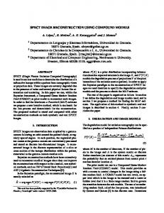
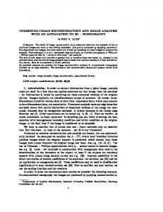
3.2. Nonlinear optical image reconstruction In this section, we present a 3D optical reconstruction with simulated measurement. The forward mesh were generated from a patient tomosynthesis scan, multiple slides of the scan were shown in Fig. 5. The forward and reconstruction mesh pair was created by truncating the initial mesh by the binary image stack of the TOMO scan at different sizes. There is not moving mesh step applied on this mesh due to the difficulties of using QHull to tessellate 3D uniform grid. For simplicity, we only use the initial mesh for reconstruction. The simulated optical properties were generated by modulating another tumor patient’s TOMO scan (shown in Fig. 6 (a)). The contrast of the tumor to the background is about 2:1. The reconstructed image slices from simulated RF measurements were shown in Fig. 6 (b). To demonstrate the importance of using geometry information from X-ray, we also reconstructed the target with a uniform grid mesh. The result is shown in Fig. 7.
Figure 5. Sample slices of a breast tomosynthesis image: (a) z = 0.1 cm, (b) z = 1.5 cm, (c) z = 3.6 cm.
0.2
0 0.05
0.02
0.04
0.06
0.08
0.1
X
0.12
0.14
0.16
0.18
0.2
0.02
0.02
0 0.05
0.04
z=4 cm
0.14
0.08
0.1
0.12
0.14
0.16
0.18
0.2
0.1
0.12
X
0.14
0.16
0.18
0.2
0 0.04 0.02
Y 0.04
0.02
0.04
0.06
0.08
0.1
0.12
0.14
0.16
0.18
0 0.04 0.02
X
0.12
0.12
0.1
0.1
0.1
0.08
0.08
0.08
Y
Y
0.12
0.08
0.06
0.06
0.04
0.04
0.04
0.02
0.02
0.02
0 0.05
Z
0.06
0.02
0.04
0.06
0.08
0.1
0.12
0.14
0.16
0.18
0.2
0 0.05
0.04
0.06
0.08
0.1
0.12
0.14
0.16
0.18
0 0.04 0.02
0.06
0.04
0.02
0.04
0.06
0.08
0.1
X
z=5.5 cm
0.14
0.08
0.18
0.1
0.12
0.14
0.16
0.18
0 0.04 0.02
X
z=5 cm
0.14
z=5.5 cm
0.12
0.12
0.12
0.12
0.1
0.1
0.1
0.1
0.08
0.08
0.08
Y
Y 0.06
0.16
0.12
0.08
0.04
0.14
z=4 cm
X
z=5 cm
0.12
z=3 cm
0.14
X
0.02
0.1
0.06
Y
0.06
0.08
0.08
X
Y 0.04
0.06
X
z=3 cm
0.02
Y 0.04
0.06
0.06
0.04
0.04
0.04
0.02
0.02
0.02
Z
0.06
0 0.05
0.02
0.04
0.06
0.08
0.1
0.12
X
0.14
0.16
0.18
0.2
0 0.05
0.04
0.06
Z
0.18
0.04
0.1
Y
0.16
0.06
Y
0.14
0.06
Z
0.12
0.12
4.50 4.00 3.50 3.00 2.50 2.00 1.50 1.00
0.08
0.1
0.12
X
0.14
0.16
0.18
0 0.04 0.02
0.06
0.04
0.02
Z
0.1
0.08
Z
0.08
0.08
Z
0.06
Z
0.02
0.1
Z
0.04
0.1
0.04
0.06
0.08
0.1
0.12
0.14
0.16
0.18
0 0.04 0.02
Z
0.06
4.50 4.00 3.50 3.00 2.50 2.00 1.50 1.00
Y
Y
0.08
0.04
z=2 cm 0.12
0.12
0.1
0.02
z=1 cm
0.14
0.12
Z
z=2 cm
0.14
Z
z=1 cm
X
Figure 6. True and recovered absorption (m−1 ) of the simulated breast.
The reconstruction result in Fig. 6 (b) correct capture the tumor and glandular area of the breast. In contrast, the case without considering the geometry (Fig. 7) generated images with significant level of artifacts, despite the fact that the relative residue of the reconstruction is low (about 3%).
4. DISCUSSIONS AND CONCLUSIONS We presented a combined X-ray/optical breast imaging system. A simple and efficient mesh generator was proposed to produce high-quality finite elements from X-ray scans. This mesh generator is conceptually simple which allows it to be easily adapted for other multi-modality scenarios. We also discussed the use of an iterative block solver and its acceleration to the forward field modeling. Numerical simulations highlighted the importance of modeling geometry boundaries of the target for image reconstruction, which further demonstrates the necessity of combining X-ray with DOT in breast imaging. In this study, we also appreciated the following problems: 1) the mesh generator is not entirely stable, a thorough understanding to the stability of this algorithm is necessary; 2) some elements closed to the boundaries may have low quality, modifications to the algorithm needs to be made to avoid this situation; 3) for 3D mesh generation, tessellation algorithm such as QHull can not properly handle
z=1 cm
z=2 cm 0.12
0.12
0.06
0.04
0.08
0.1
0.12
0.14
0.16
0.18
0 0.04 0.02
0.04
0.02
0.04
0.06
0.08
0.1
X
0.12
0.14
0.16
0.18
0 0.04 0.02
X
z=3 cm
z=4 cm 0.12
0.1
0.1
0.08
0.08
Y
Y
0.12
0.06
0.06
0.04
0.04
0.02
0.04
0.06
0.08
0.1
0.12
0.14
0.16
0.18
0.02
Z
0 0.04 0.02
0.04
0.06
0.08
0.1
X
0.12
0.14
0.16
0.18
0 0.04 0.02
X
z=5 cm
z=5.5 cm 0.12
0.1
0.1
0.08
0.08
Y
Y
0.12
0.06
0.06
0.04
0.04
0.02
0.04
0.06
Z
0.06
0.06
0.08
0.1
0.12
X
0.14
0.16
0.18
0.02
Z
0 0.04 0.02
0.04
0.06
0.08
0.1
0.12
0.14
0.16
0.18
0 0.04 0.02
Z
0.04
0.08
Z
0.02
0.1
Y
Y
0.08
4.50 4.00 3.50 3.00 2.50 2.00 1.50 1.00
Z
0.1
X
Figure 7. Recovered absorption (m−1 ) without geometric modeling.
rectangular grid at the beginning of the moving mesh process, an improved tessellation algorithm should be considered.
REFERENCES 1. A. P. Gibson, J. C. Hebden, and S. R. Arridge, “Recent advances in diffuse optical imaging,” Phys. Med. Biol. 50, pp. R1–R43, 2005. 2. J. C. Hebden, S. R. Arridge, and D. T. Delpy, “Optical imaging in medicine: I. experimental techniques,” Phys. Med. Biol. 42, pp. 825–840, 1997. 3. S. R. Arridge and J. C. Hebden, “Optical imaging in medicine: Ii. modelling and reconstruction,” Phys. Med. Biol. 42, p. 841C853, 1997. 4. B. Brooksby, H. Dehghani, B. W. Pogue, and K. D. Paulsen, “Near infrared (NIR) tomography breast image reconstruction with a priori structural information from MRI: algorithm development for reconstructing heterogeneities,” IEEE Journal of Selected Topics in Quantum Electronics (Special issue on Lasers In Biology and Medicine) 9, pp. 199–209, 2003. 5. Q. Zhang, T. J. Brukilacchio, A. Li, J. Stott, T. Chaves, E. Hillman, T. Wu, M. Chorlton, E. Rafferty, R. H. Moore, D. B. Kopans, and D. A. Boas, “Coregistered tomographic x-ray and optical breast imaging: initial results,” Journal Biomed Optics 10, p. 024033, 2005. 6. P. Persson and G. Strang, “A simple mesh generator in matlab,” SIAM Review 46(2), pp. 329–345, 2004. 7. D. B. Kopans, Breast Imaging, Lippincott Williams & Wilkins, 1998. 8. C. B. Barber, D. P. Dobkin, and H. Huhdanpaa, Tech. Report No. GCG53, The Geometry Center, University of Minnesota, 1993. 9. K. D. Paulsen, P. M. Meaney, M. J. Moskowitz, and J. M. S. Jr., “A dual mesh scheme for finite element based reconstruction algorithms,” IEEE Trans. Med. Imag. 14, pp. 504–514, 1995. 10. Q. Fang, Ph.D. Thesis: Computational methods for microwave medical imaging, Dartmouth College, 2005. 11. T. A. Davis, “Algorithm 832: Umfpack - an unsymmetric-pattern multifrontal method with a column preordering strategy,” ACM Trans. Math. Software 30(2), pp. 196–199, 2004. 12. J. W. Demmel, S. C. Eisenstat, J. R. Gilbert, X. S. Li, and J. W. H. Liu, “A supernodal approach to sparse partial pivoting,” SIAM J. Matrix Analysis and Applications 20(3), pp. 720–755, 1999. 13. R. W. Freund, “Conjugate gradient type methods for linear systems with complex symmetric coefficient matrices,” SIAM J. Sci. Statist. Comput. 13, pp. 425–448, 1992. 14. W. E. Boyse and A. A. Seidl, “A block QMRmethod for computing multiple simultaneous solutions to complex symmetric systems,” SIAM J. Sci. Comput. 17, pp. 263–274, 1996. 15. Q. Fang, P. M. Meaney, S. D. Geimer, and a. K. D. P. A. V. Streltsov, “Microwave image reconstruction from 3D fields coupled to 2D parameter estimation,” IEEE Trans. Med. Imag. 23, pp. 475–484, Apr 2004.