Evolutionary Hierarchical Dirichlet Processes for ... - Semantic Scholar

Evolutionary Hierarchical Dirichlet Processes for Multiple Correlated Time-varying Corpora Jianwen Zhang† ,

Yangqiu Song‡ ,

Changshui Zhang† ,

Shixia Liu‡

†

State Key Laboratory of Intelligent Technology and Systems † Tsinghua National Laboratory for Information Science and Technology † Department of Automation, Tsinghua University, Beijing 100084, China ‡ IBM Research – China, Beijing, China †

{jw-zhang06@mails,zcs@mail}.tsinghua.edu.cn; ‡ {yqsong,liusx}@cn.ibm.com

ABSTRACT Mining cluster evolution from multiple correlated time-varying text corpora is important in exploratory text analytics. In this paper, we propose an approach called evolutionary hierarchical Dirichlet processes (EvoHDP) to discover interesting cluster evolution patterns from such text data. We formulate the EvoHDP as a series of hierarchical Dirichlet processes (HDP) by adding time dependencies to the adjacent epochs, and propose a cascaded Gibbs sampling scheme to infer the model. This approach can discover different evolving patterns of clusters, including emergence, disappearance, evolution within a corpus and across different corpora. Experiments over synthetic and real-world multiple correlated timevarying data sets illustrate the effectiveness of EvoHDP on discovering cluster evolution patterns.

Categories and Subject Descriptors I.2.6 [Artificial Intelligence]: Learning; I.5.3 [Pattern Recognition]: Clustering; G.3 [Probability and Statistics]: Nonparametric statistics; H.2.8 [Database Management]: Database applications—Data mining

General Terms Algorithms; Experimentation

Keywords Multiple correlated time-varying corpora, clustering, mixture models, Bayesian nonparametric methods, Dirichlet processes

1.

INTRODUCTION

Nowadays, we are surrounded by overwhelming quantities of textual materials from various heterogenous corpora (e.g., news, blogs) everyday. The themes in these corpora are usually similar, however, diversity also exists. For example, news typically has more discussions on society, politics, and economics than blogs which might focus more on personal life. Even within a corpus, the

Permission to make digital or hard copies of all or part of this work for personal or classroom use is granted without fee provided that copies are not made or distributed for profit or commercial advantage and that copies bear this notice and the full citation on the first page. To copy otherwise, to republish, to post on servers or to redistribute to lists, requires prior specific permission and/or a fee. KDD’10, July 25–28, 2010, Washington, DC, USA. Copyright 2010 ACM 978-1-4503-0055-1/10/07 ...$10.00.

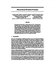
Figure 1: The cluster “financial crisis” discovered by EvoHDP in 103,986 articles crawled from three types of web corpora: blogs, news and message boards. Each corpus is represented by a colored stripe. The height of a stripe is the proportion of the cluster in corresponding corpus. For each corpus, the top keywords of this cluster in each month are placed on the stripe, where the size of a keyword encodes its frequency in the cluster. The popularity of this cluster in each corpus varied over time. In addition, the cluster was first active in blogs and then became popular in news and message boards. popularity of themes may also vary over time, and some of them may first appear in blogs, and then spread to news and message boards. Fig. 1 shows a real example of an evolving document cluster about “financial crisis” in three types of web corpora, including blogs, news and message boards. To better understand the complex data, users not only want to examine the document clusters, but also want to discern the cluster evolution patterns over time and across corpora. Specifically, from multiple correlated time-varying corpora, it is desirable to discover the following patterns: (1) clusters within each corpus at each time epoch, (2) shared clusters among different corpora at each epoch, (3) evolving patterns of clusters within a corpus, and (4) evolving patterns of clusters across corpora over time. However, it is challenging to learn cluster evolution patterns from such complex data. The first challenge is how to model the clusters both across different corpora and over time. On the one hand, we need a single integrated model for all corpora to set up a global bookkeeper of clusters, otherwise we can not easily discern the evolution of a cluster across corpora over time. On the other hand, different corpora may share some clusters while also having their distinctive clusters. Hence the commonality and diversity should be both reflected in the single integrated model. The second challenge is how to model the time dependencies in the multiple corpora setting. It is very common the themes of a corpus evolves slowly along time, and thus the clustering patterns of adjacent time epochs usually exhibit strong correlations. Incorporating these correlations

into the model in the multiple corpora setting is nontrivial. The last challenge is how to determine the cluster numbers. In time varying text data, a cluster may emerge and disappear. Consequently, the cluster numbers may change through time. It is awkward to require users to specify a cluster number at each time epoch for each corpus. Therefore a mechanism is preferred to automatically determine all the numbers of clusters. The traditional clustering approaches deal with a single static data corpus. Hence the direct use of a general global clustering model on all data may fail to represent the diversity both over time and across different corpora. Beyond the classical clustering approaches, the most recent efforts only focus on tackling two sub problems. One is learning from multiple correlated text corpora, which aims to discover the related content across different text corpora as well as the distinctive information in each corpus [22, 26, 17]. Another is learning from a time-varying data corpus, which aims to discover the evolving patterns in the corpus as well as the snapshot clusters at each time epoch [3, 8, 9, 1, 16]. Both types of approaches are not sufficient to tackle the above challenges. To deal with above challenges, in this paper, we propose an evolutionary hierarchical Dirichlet process (EvoHDP) model, which extends the hierarchical Dirichlet process (HDP) [22] to a time evolving scenario. In EvoHDP, each HDP is built for multiple corpora at each time epoch, and the time dependencies are incorporated into adjacent epochs under the Markovian assumption. Specifically, the dependency is formulated by mixing two distinct Dirichlet processes (DPs). One is the DP model for the previous epoch, and the other is an updating DP model. To infer the EvoHDP model, we also propose a cascaded Gibbs sampling scheme. The proposed EvoHDP model can effectively discover cluster evolution patterns over time and across corpora. Moreover, the cluster numbers can automatically be determined due to the infinity property of DP.

2.

RELATED WORK

In this section, we briefly introduce three categories of work related to this paper, including learning from multiple correlated data corpora, learning evolution patterns from a time-varying corpus, and some initial efforts involving multiple dynamic data. In the research of learning from multiple correlated data corpora, HDP is a milestone [22]. It extended DP [2, 23] to model multiple correlated data corpora. In HDP, each data corpus is modeled by an infinite DP mixture model, and the infinite set of mixing clusters is shared among all corpora. Later works [16, 6] relax the assumption of HDP and incorporate more correlations between different corpora. Besides HDP, other efforts [4, 19, 26, 17] on this research topic are devoted to the extensions of the Latent Dirichlet Allocation (LDA) topic model [5]. However, none of them consider the problem of automatically determining the cluster/topic numbers. In fact, as pointed out in [22], HDP can be used as an LDA-based topic model, where the number of clusters can be automatically inferred from data. Therefore, HDP is more practical when users have little knowledge about the content to be analyzed. In the research of learning evolutionary clusters from a timevarying corpus, evolutionary clustering [8, 9, 32, 1, 30, 31] is a new research topic. Evolutionary clustering aims to preserve the smoothness of clustering results over time, while fitting the data of each epoch. Among the above works, the approaches in [1, 30, 31] utilized DP to automatically determine the cluster numbers. In fact, incorporating time dependencies into DP mixture models is a hot topic in the research of Bayesian nonparametric [20, 10, 7, 16, 15, 14]. Moreover, some works have focused on extending LDA to dynamic topic models [3, 27, 25]. We noted that even though the title

of [16] is similar to this paper, it actually presents an evolutionary DP mixture model for a single dynamic corpus. To the best of our knowledge, there are four works that seemingly involve multiple time-varying data but actually handle different problems [28, 29, 11, 21]. Wang et al. [28] focused on detecting the simultaneous busting of some topics in multiple text streams. They did not concentrate on the evolving patterns but only the busting behavior of topics. Wang et al. [29] extended [28] to extract common topics from multiple text streams. They regarded that the underlying models of all streams are the same except that time delays exist between different streams. Hence they adjusted the timestamps of of all documents to synchronize multiple streams and then learned a common topic model. Their assumption pays more attention to aligning topics of different streams and thus degenerates the topic diversity among different streams. Leskovec et al. [11] focused on tracking the spreading behaviors of short phrases (or “memes”) across the web to represent news cycles. Although memes act as signatures of clusters/topics, they are not enough to represent clusters/topics as the context information is lost. Tang et al. [21] worked on the dynamic multi-mode network with several types of actors. They aimed to provide a partition for each type of actors at each time epoch. There are two typical features in their problem: (1) the data to be handled is relational data, i.e., linkages between actors are required; (2) the partitions over time should be on a same set of actors while relationships among them vary over time. None of the above four works attempted to discover the cluster evolution over time and across corpora. On the contrary, this is exactly the focus of this paper. In addition, none of them handled the problem of automatically determining the cluster/topic numbers, which is one of the major considerations of our work.

3.

PRELIMINARIES

In this section, we briefly introduce DP and HDP. A DP can be considered as a distribution of a random probability measure1 G, and we write G ∼ DP(α0 , G0 ), where α0 is a positive concentration parameter, and G0 is a base measure. Sethuraman [18] showed that a measure G drawn from a DP is discrete, by the following stick-breaking construction: X∞ i.i.d. {φk }∞ πk δφk . (1) k=1 ∼ G 0 , π ∼ GEM (α0 ) , G = k=1

The discrete set of atoms {φk }∞ k=1 are drawn from the base measure, andQGEM (α0 ) refers to such a process: π˜ k ∼ Beta(1, α0 ) , πk = π˜ k k−1 ˜ i ) . We use boldface π = (πk )∞ i=1 (1 − π k=1 to represent the vector, which will be followed in the rest of the paper. δφk is a probability measure concentrated at φk . After observing draws θ1 , . . . , θn−1 from G, the posterior of G is still a DP ! mk δφk + α0 G0 , (2) G|θ1 , . . . , θn−1 ∼ DP α0 + n − 1, α0 + n − 1 where mk is the number of draws in {θi }n−1 i=1 taking the same value φk . This posterior preserves the possibility of drawing a new distinct value from G0 but puts more concentration on observed values. HDP uses multiple DPs to model multiple correlated corpora. In HDP, a global measure G0 is drawn from a DP (γ, H), with concentration parameter γ and base measure H. Then, a set of measures {G j } j is drawn from a DP with base measure G0 . Each G j models the corpus j . Such a process is summarized as i.i.d.

G0 ∼ DP (γ, H) , G j |G0 , α0 ∼ DP (α0 , G0 ) . (3) Given the global measure G0 , G j ’s are conditionally dependent. nj Having G j , n j data samples {x ji }i=1 in each corpus j are drawn from 1

In general, we can regard the measure as a distribution.

 γ    H G0 

 α0  

Gj

θji

xji

nj

J

 α0  γ    πj

β

zji

nj

J

(a)

xji

  H   φk

K(∞)

(b)

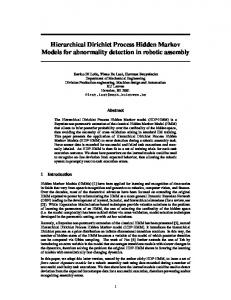
Figure 2: Graphical representation for HDP: circles denote random variables, oval nodes denote parameters, shaded nodes denote observed variables, and plates indicate replication. (a) HDP. (b) The stick-breaking construction of HDP.

 γ t−1

t−1 G0

  α0t−1

Gt−1 j t−1 θji

xt−1 ji n

 H  

ξ

G

 γt

wt

vjt

t  G0

  α0t

 γ t+1

vjt+1

  α0t+1

Gtj t θji

nt j

t+1 θji

n

Jt

i.i.d.

{θ ji }i ∼ G j , x ji ∼ F(x|θ ji ), (4) where F(x|θ ji ) is a distribution parameterized by θ ji to generate x ji , e.g., that of an exponential family. Eqs. (3) and (4) together define the hierarchical Dirichlet process mixture model2 . The graphical representation for an HDP is described in Fig. 2(a). P Moreover, according to Eq. (1), G0 has the form G0 = ∞ k=1 βk δφk , i.i.d. where φk ∼ H , β ∼ GEM(γ) . Then it is shown in [22] that G j can be constructed Xas∞ Gj = π jk δφk , π j | β, α0 ∼ DP (α0 , β) , (5) k=1

which means that different corpora share the same set of distinct atoms [22]. This is the stick-breaking construction of HDP, and the corresponding graphical model is shown in Fig. 2(b).

4.

EVOLUTIONARY HDP

In this section, we begin with the introduction of the EvoHDP model, and then show how to infer the model using a proposed Gibbs sampling technique. We first introduce the data settings and some notations which are useful for subsequent discussions. There are J corpora varying over T time epochs. Considering the possibility that no data observed for some corpora at an epoch, we denote the number of corpora at epoch t is J t . At each epoch t , there are ntj data samples in corpus j , and we denote a data sample (e.g., a document3 ) as xtji . We assume the underlying model to generate xtji for corpus j at epoch t is an infinite mixture model Z ptj (x|Gtj ) =

Gtj (θ) f (x|θ)d θ ,

P t where Gtj = ∞ k=1 π jk δφk and f is the density of a distribution F(x|θ). We call the density parameterized by a distinct atom φk as a mixing component, which describes a cluster.4

4.1

Model

We model the multiple correlated time-varying corpora as a series of HDPs with time dependencies, as shown in the graphical presentation of Fig. 3(a). Specifically, at each time epoch t, we use an HDP to model the multiple correlated corpora at that epoch and then put time dependencies between adjacent epochs based on the Markovian assumption. To build an overall bookkeeping of components for all epochs, we let these HDPs share an identical discrete base measure G, and G is drawn from DP(ξ, H) with H as the base measure. We call G the overall measure. Moreover, for an HDP to 2 We just call “hierarchical Dirichlet process mixture model” as HDP for short in this paper. 3 Generally a data sample can be quite different. For example, when using HDP to formulate LDA topic model, a data sample is a word. 4 When x represents a word, and F(x|θ) is a multinomial distribution over a finite word vocabulary, the distribution F is often regarded as a “topic” [5].

ν

vjt

  α0t

t+1 j J t+1

wt+1

vjt+1

  α0t+1

πjt t zji

xt−1 ji t−1 j J t−1

 β γ t+1

  βt γt

wt

 H

t+1

πjt+1 t+1 zji

xt+1 ji

xtji

n

(a) the following mixture model

β

π t−1   j t−1 α 0

t−1 zji

Gt+1 j

xt+1 ji

xtji

t−1 j J t−1

  γ t−1

t+1 G0

wt+1

t−1

 ξ

nt j

n

Jt

φk

t+1 j J t+1

K

(b)

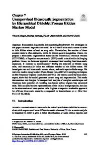
Figure 3: The graphical representation for the EvoHDP model. (a) The original representation. (b) The stick-breaking construction. model the corpora at epoch t, we use Gt0 to denote the global measure at that epoch, and call it the snapshot global measure. Then, the local measure Gtj for the j-th corpus at time epoch t is called the snapshot local measure. In this way, an EvoHDP has one more layer than the original HDP [22]. The key issue of EvoHDP is how to incorporate time dependencies between adjacent epochs. We introduce two types of dependencies into different layers in EvoHDP to model the different evolving manner. In the following we will interpret this model stepby-step to explain why we use this scheme and how it would be useful. The first is the dependency of snapshot global measure Gt0 on t Gt−1 0 . Since G 0 is the measure for the components in all corpora at time t, the difference between Gt0 and Gt−1 0 reflects the evolving of the global components in all corpora. We call this global time dependency . The second is the time dependency within a corpus, i.e., the det pendency of the snapshot local measure Gtj on Gt−1 j . Since G j is the measure for the components within corpus j at time epoch t, the difference between Gtj and Gt−1 reflects the evolving of comj ponents within the corpus j. Then we call this intra-corpus time dependency. In Fig. 3(a), we use dashed lines to represent the second type of dependencies, since in some cases (e.g. in HDP based LDA), there are no intra-corpus dependencies. The generation process of EvoHDP is as follows. 1. Draw an overall measure G ∼ DP(γ, H). G plays a role of the overall component bookkeeping for all corpora at all epochs. 2. For each epoch t : 2.1. Draw the snapshot global measure Gt0 according to the overall measure G and the previous snapshot global measure Gt−1 0 :   t t t t−1 t G0 ∼ DP γ , w G0 + (1 − w )G . (6) t

2.2. Draw the snapshot local measures {Gtj } Jj=1 . Each Gtj for corpus j at epoch t is drawn according to the snapshot global measure Gt0 and the previous snapshot local measure Gt−1 j :   t t Gtj ∼ DP αt0 , vtj Gt−1 (7) j + (1 − v j )G 0 . nt

t

j J 2.3. For data samples {{xtji }i=1 } j=1 , draw the parameters of the component densities and generate the data samples:

i.i.d.

θtji ∼ Gtj , xtji ∼ F(x|θtji ), where F(x|θtji ) is a distribution parameterized by θtji , e.g., that from an exponential family. Compared to the original HDP model, two levels of time dependencies are incorporated in by Eq. (6) and Eq. (7). When we set all wt and vtj to zero, the EvoHDP is a three-layer HDP.

π ˆ jt

  α0t+1

β t+1

  α0t πjt

vjt+1

t+1 kjτ

t+1 Tj•

ntj

nt+1 j

(a)

β t+1

π ˆ jt

  ut+1 j v t+1 α0t πjt j

t+1 τji

t+1 zji

t zji

  γ t+1

ν

t zji

ntj

t+1 kjτ

t+1 kjτ

t→t+1 Tj•

0→t+1 Tj•

t β t−1 w β t   γt

wt+1

t+1 km

M•t+1 t+1 kjτ

t kjτ 0→t Tj•

t+1 Tjk

=

t→t+1 Tjk

+

0→t+1 Tjk

ut+1

mt+1 jτ

t+1 km

M•0→t+1

M•t→t+1

0→t Tj•

J t+1

t+1 km

wt+1

t kjτ

Jt

(a)

(b)

1 − wt+1

β t−1 w β t   γt

0→t+1 Tj•

Jt

ν t

Mkt+1 = Mkt→t+1 + Mk0→t+1

(b)

Figure 4: The generation mechanism of Gt+1 j . (a) A part insight into the generation process of restaurant j at epoch t + 1. (b) The generation of tables of restaurant j at epoch t + 1.

Figure 5: The generation mechanism of Gt+1 0 . (a) A part insight into the generation process of the snapshot global measure. (b) The generation of meta-tables of the franchise at epoch t + 1.

Following the convention of DP related models [22, 24, 16], we will also provide other two perspectives and a restaurant-metaphor for the EvoHDP. They help us better understand the model and lay the foundations of the inference scheme introduced in Sec. 4.4.

distribution on tables. We can explain Eq. (10) as a peculiar way of dish serving in a restaurant. First, waiters place infinite number of tables. On each table τ, a dish kt+1 jτ is selected from the local table-dish menu πˆ t+1 by waiters. Then, when a customer i enters j in restaurant j, he selects a table τt+1 from the local customer-table ji t+1 on the ) and enjoys the dish kt+1 (with probability u menu ut+1 t+1 j jτt+1 jτ

4.2

The Stick-Breaking Construction

According to the stick-breaking construction (Eq. (1)) of DP, we can write the explicit form of G: X∞ G= νk δφk , ν ∼ GEM(ξ) . k=1

Consequently, according to Eqs. (6) and (5), G0 has the form X∞   Gt0 = βtk δφk , βt ∼ DP γt , βˆ t ,

(8)

where βˆ t = wt βt−1 + (1 − wt )ν . Similarly, we can also write the form of Gtj as X∞   Gtj = πtjk δφk , πtj ∼ DP αt0 , πˆ tj ,

(9)

k=1

k=1

t t where πˆ tj = vtj πt−1 j + (1 − v j )β . In this way, we obtain the stick-breaking construction for EvoHDP, which is shown in Fig. 3(b), where ztji is the index of the component emitting xtji . According to this perspective, the EvoHDP provides a prior in which the snapshot models {Gt0 }t , {Gtj }t, j of all corpora at all epochs share the same infinite set of mixing components {φk }∞ k=1 . The differences among these snapshot models lie in the mixing weights.

4.3

Hierarchical Infinite Mixture Model and A Restaurant Franchise Metaphor

Based on the stick-breaking construction for a DP, if we continue to use the stick-breaking constructions to represent πtj and βt drawn from the two DPs in Eqs. (8) and (9), we obtain the hierarchical infinite mixture model of EvoHDP. This perspective clearly interprets the generation mechanism of EvoHDP. We begin with the metaphor following the Chinese restaurant franchise (CRF) for HDP [22]. A corpus j is called a restaurant, and a global atom k is called a dish. We use a day to refer to a time epoch. We focus on the generation of component indicator ztji . Having ztji , the left generation process of xtji is straightforward, which is drawn from F(x|φztji ).

4.3.1

Generation of Snapshot Local Measure Gtj

We first show thePgeneration mechanism of each snapshot lot+1 cal measure Gt+1 = ∞ k=1 π jk δφk , i.e., the behavior of restaurant j j t+1 ˆ t+1 in day t + 1. Since π j is drawn from DP(αt+1 j ) as shown in 0 ,π Eq. (9), we can represent this DP using the stick-breaking construction as X ∞ i.i.d. t+1 t+1 ˆ j , ut+1 πt+1 = ut+1 ∼ GEM(αt+1 j jτ δkt+1 , {k jτ }τ ∼ π j 0 ), (10) τ=1

jτ

which is illustrated in Fig. 4(a). We call τ a table, then ut+1 is a j

ji

ji

t+1 table. Consequently, the component indicator zt+1 ji = k jτt+1 . Moreji

over, πt+1 plays the role of the local customer-dish menu, which j indicates the customers’ preference on dishes in day t + 1 . We then explain how a dish is placed on a table by the waiter. i.i.d. ˆ t+1 From Eq. (10), we see that {kt+1 jτ }τ ∼ π j , i.e., a dish is drawn t from the local table-dish menu πˆ t+1 . Notice that πˆ t+1 = vt+1 j j j π j +(1− t+1 t vt+1 )β is a mixture of two menus, where π is the local customerj j dish menu in this restaurant yesterday and βt+1 is the global franchise menu of current day recommended by the franchise manager. Then for a table τ, a waiter select a dish kt+1 jτ from yesterday’s local customer-dish menu πtj with probability vt+1 j while from current day’s global franchise menu βt+1 with probability 1 − vt+1 j . This means in the franchise, a restaurant designs its localized menu by considering both yesterday’s local taste and current day’s franchise menu. Obviously, it is possible that multiple tables have a same dish. In restaurant j in day t + 1, we denote the number of tables with dish k as T t+1 jk . Then the total number of tables in restaurant j in day P t+1 t + 1 is denoted as T t+1 k T jk . Then for a dish k, among the j• = t→t+1 T t+1 tables whose dishes are selected from jk tables, there are T jk yesterday’s local customer-dish menu πtj , and T 0→t+1 tables whose jk dishes are selected from current day’s global franchise menu βt+1 . t→t+1 Then, ∀ k, we have T t+1 + T 0→t+1 . This mechanism is jk = T jk jk shown in Fig. 4(b).

4.3.2

Generation of Snapshot Global Measure Gt0

Then we showPthe generation mechanism of the snapshot global t measure G0t+1 = ∞ k=1 βk δφk , i.e., how the franchise manager recommends the global franchise menu βt+1 to all restaurants. The procedure is explained in Fig. 5(a). Since βt+1 is drawn from DP(γt+1 , βˆ t+1 ) as shown in Eq. (8), βt+1 can also be represented using the stickbreaking construction as X∞ i.i.d. βt+1 = umt+1 δkt+1 , {kmt+1 }m ∼ βˆ t+1 , ut+1 ∼ GEM(γt+1 ). (11) m=1

m

We call each m a metatable, then ut+1 is a distribution on metatables. The manager has infinite number of empty metatables beforehand and he selects a dish kmt+1 for each metatable m from the metatable-dish menu βˆ t+1 of day t + 1 . Remind that when a waiter in restaurant j place a table τ, with probability 1−vt+1 j , he selects the t+1 dish kt+1 according to the global franchise menu β . Now he just jτ

need to select a metatable mt+1 jτ according to the waiter-metatable menu ut+1 , and then the dish kmt+1t+1 on the metatable is the one he jτ

should select. Hence the global franchise menu βt+1 also plays the role of the waiter-dish menu, which indicates how a waiter selects dishes for tables. The dishes on the metatables of the franchise in day t + 1 also come from two menus, i.e., the yesterday’s global franchise menu βt and an overall menu ν. The overall menu ν reflects common taste of the franchise. It is also possible that different metatables have a same dish and we denote the number of metatables with dish k as Mkt+1 . Among the Mkt+1 metatables, there are Mkt→t+1 metatables whose dishes are selected from yesterdays’ franchise menu, and Mk0→t+1 metatables whose dishes are selected from the overall menu ν . Then ∀ k , we have Mkt→t+1 = Mkt→t+1 + Mk0→t+1 .

4.4

A Cascaded Gibbs Sampler

Sampling ν According to the generation of metatables introduced in Fig. 5(b), P what are drawn from the overall measure G = ∞ k=1 νk δφk are the dishes on the metatables of all days designed by the franchise manager. We P denote the number of all these metatables with dish k as Mk = t Mk0→t P , and the total number of metatables drawn from G as M• = k Mk . As G ∼ DP(ξ, H), assume we have known the count variables {Mk }k , according to the property Eq. (2), the posterior of G is also a DP:   PK H + k=1 Mk δφk   K  , G ξ, H, {Mk }k=1 ∼ DP ξ + M• , ξ + M• where K is the number of distinct dishes on all metatables. According to Sec. 5.2 of [22], G can be represented as XK G= νk δφk + νu Gu , Gu ∼ DP(ξ, H) (12) 4.4.1

k=1

ν = (ν1 , . . . , νK , νu ) ∼ Dirichlet (M1 , . . . , MK , ξ) . (13) This augmented representation reformulates original infinite vector ν to an equivalent finite one with length K + 1. Then ν is sampled from the Dirichlet distribution of Eq. (13). Notice that in the following, Gt0 and Gtj are also represented using above augmented representation as XK XK Gt0 = βtk δφk +βtu Gu , Gtj = πtjk δφk +πtju Gu , Gu ∼ DP(ξ, H). k=1

Then βt and πtj are both represented as finite vectors  
βt = βt1 , . . . , βtK , βtu , πtj = πtj1 , . . . , πtjK , πtju .

4.4.2

where α˜ t0 = αt0 + N tj• , and  1  t t t t π˜ tjk = t αt0 vt πt−1 jk + α0 (1 − v )βk + N jk , α˜ 0  1  t t t π˜ tju = t αt0 vt πt−1 jk + α0 (1 − v )βk . α˜ 0

4.4.3

The hierarchical infinite mixture model and the restaurant franchise metaphor actually define a Gibbs sampling scheme for EvoHDP. We can derive a cascaded Gibbs sampling procedure by sequentially sampling following variables.

k=1

where γ˜ t = γt + T•t , and  1  t t t β˜ tk = t γt wt βt−1 k + γ (1 − w )νk + Tk , γ˜  1  t β˜ u = t γt wt βut−1 + γt (1 − wt )νu . γ˜ The sampling of πtj is similar to that of βt :      πtju , πtj1 , . . . , πtjK ∼ Dir α˜ t0 · π˜ tju , π˜ tj1 , . . . , π˜ tjK ,

Sampling βt and πtj

According to Fig. 5(b),Pwhat are drawn from β include two parts. 0→t 0→t One part is the T •• = j,k T 0→t dishes on the T •• tables in all jk t→t+1 restaurants of day t. The second part is the M• dishes on the M•t→t+1 metatables of next day t + 1 . We call all these tables and metatables drawn from βt as pseudo-tables. We denote the number 0→t of pseudo-tables withthe same dish k as Tkt , then Tkt = T •k +  t→t+1 t t ˆt Mk . As β ∼ DP γ , β , and assuming we have obtained the count variables {Tkt }k , the posterior of βt is also a DP. Similar to Eq. (13), βt can also be sampled from a Dirichlet distribution   
βtu , βt1 , . . . , βtK ∼ Dirichlet γ˜t · β˜ tu , β˜ t1 , . . . , β˜ tK , (14) t

(15) (16)

(17)

(18) (19)

Sampling ztji

Given πtj , sampling ztji is straightforward:       p ztji = k xtji , · · · ∝ p ztji = k πtj p xtji ztji = k, · · · , (20) where k ∈ {1, . . . , K, u} . u refers to the index for the new component as introduced in Eq. (12). When k = u is sampled, we add a new component into the bookkeeping. In Eq. (20),  component  the first item is a prior p ztji = k πtj = πtjk and the second item is a likelihood    Z    (21) f xt φ p φ X k , H dφ , p xt zt = k, . . . = ji

ji

ji

k

k

¬t, ji

k

k X¬t, ji

where is the set of all the samples having been assigned to component k, other than xtji .

4.4.4

Sampling T tjk and Mkt

As described in Sec. 4.4.1 and Sec. 4.4.2, the posterior of ν, βt and πtj depend on the count variables T tjk and Mkt . P Remind that the count variable T tj• = k T tjk is the number of all tables in restaurant j at epoch t. These tables are occupied by the N tj = ntj + T t→t+1 pseudo-customers. A pseudo-customer with j• dish k must have sat at a table with dish k. Hence ∀k, the N tjk = ntjk + T t→t+1 pseudo-customers cluster into T tjk tables. As shown jk in [22], given N tjk , the table number T tjk can be sampled from a Chinese Restaurant Process (CRP)   t t t t−1 t t t t T tjk βtk , πt−1 jk , N jk ∼ CRP α0 v j π jk + α0 (1 − v j )βk , N jk . Notice that N tjk = ntjk +T t→t+1 . As ntjk is the number of customers jk with dish k, it can be counted from the component assignments. To know N tjk , we also need to know T t→t+1 , which depends on T t+1 jk jk in turn. Thus the variable T tjk can be sampled from following recursive procedure:     T t→t+1 , T 0→t+1 ∼ Multinomial T t+1 (22) jk jk , [p, 1 − p] jk N tjk = ntjk + T t→t+1 jk   t t t−1 t t t t T jk βk , π jk , N tjk ∼ CRP αt0 vtj πt−1 jk + α0 (1 − v j )βk , N jk , where p =

t vt+1 j π jk t+1 t+1 t (1−vt+1 j )βk +v j π jk

(23) (24)

.

Similarly, we obtain the recursive sampling procedure for Mkt :     Mkt→t+1 , Mk0→t+1 ∼ Multinomial Mkt+1 , [q, 1 − q] (25) 0→t Tkt = T •k + Mkt→t+1   t t t−1 t t t Mkt νk , βt−1 k , Tk ∼ CRP γ w βk + γ (1 − w )νk , Tk ,

where q =

wt+1 βtk (1−wt+1 )νk +wt+1 βtk

.

(26) (27)

4.4.5

Sampling Hyper-parameters

The concentration parameters of DPs, i.e., ξ, {γt } and {αt0 }, can also be sampled by putting a vague gamma prior on them ξ ∼ Ga(aξ , bξ ), γt ∼ Ga(aγ , bγ ), αt0 ∼ Ga(aα , bα ). (28) The sampling method is the same as that in [22]. Moreover, the time dependency parameters wt and vtj can be taken as controlling parameters or also sampled using the method in [16] by putting a Beta prior for them and sampling from the posterior. According to the sampling method for groups of variables described above, there are recursive dependencies along hierarchies and time epochs. We follow the dependencies of different sets of variables and design a cascaded Gibbs sample scheme. The procedure is summarized in Algorithm 1. Algorithm 1 A cascaded Gibbs sampling scheme (one iteration) 1: for t = T to 1 do 2: for j = 1 to J t do 3: Sampling Z tj according to Sec. 4.4.3. , and T tjk 4: ∀k = 1, . . . , K, sampling count variables T t→t+1 , T 0→t+1 jk jk according to Eq. (22-24). end for ∀k = 1, . . . , K, sampling count variables Mkt→t+1 , Mk0→t+1 , and Mkt according to Eq. (25-27). 7: end for 8: Sampling concentration parameters ξ, γt and αt0 . 9: Sampling ν according to Sec. 4.4.1. 10: for t = 1 to T do 11: Sampling βt according to Sec. 4.4.2. 12: for j = 1 to J t do 13: Sampling πtj according to Sec. 4.4.2. 14: end for 15: end for

5: 6:

4.5

Global and Local Components

We not only need the component assignments Z, but also the component parameters {φk }. As introduced in Eq. (21), {φk } have been integrated out in the sampling process. Having assignments Z, we can obtain the posterior of a φk :     p φ {xt |zt = k, ∀ t, j, i}, H ∝ p (φ |H) p {xt |zt = k}|φ . k

ji

k

ji

ji

ji

k

This distribution is a “global” one conditioned on data of all corpora from all epochs. In textual data, it denotes a global component k in the entire textual collection. If we limite the data in a corpus j at epoch t, we also obtain the posterior of φk as a local component     p φ {xt |zt = k, ∀ i}, H ∝ p (φ |H) p {xt |zt = k, ∀ i}|φ . k

ji

ji

k

ji

ji

k

This is the component k as a local one in corpus j at epoch t.

5.

EXPERIMENTS ON SYNTHETIC DATA

In this section, we use a synthetic data set from mixtures of multinomial distributions to test our approach.

5.1

Data

The data set consists of three time-evolving corpora covering 5 time epochs. Hence ∀t, J t , the number of corpora at epoch t, is 3. There are totally K = 8 components (dishes) involved in all corpora. Each dish k is a 2-dimensional multinomial distribution F(x|φk ) = Multinomial(x; φk ), with density PD D xd ! Y xd φk,d , f (x|φk ) = Qd=1 D d=1 xd ! d=1 where x is a D-dimensional nonnegative integer P vector, and φk is a D-dimensional nonnegative real vector with d φk,d = 1. Here

P D = 2 and we set d xd = 200. All the φk ’s are listed in Tab. 1. Each corpus j at epoch t is a uniform mixture of 3 tables, and each table τ is associated with a dish indexed by ktjτ . We denote the dish associated with table τ as ktjτ . Hence this local model can be represented by   X3 1 Multinomial x; φktjτ . ptj (x) = τ=1 3 Then ntj samples are drawn from this mixture model, which compose the corpus j at epoch t. More details of the data set are shown in Tab. 1. In the conjunction area of “Tables (ktj1 , ktj2 , ktj3 )”, the triple at row t and column j are the three dish indices to compose the local mixture model. In such a data set, different corpora overlap on some components, and the underlying models evolve over time.

5.2

Evaluation Criteria

We introduce several numerical criteria to evaluate two types of performances. The first type is the static performance on fitting training data and predicting held-out data. The second type is the temporal performance on preserving correlation between epochs, including the correlation within a corpus and that across different corpora.

5.2.1

Static Criteria

Two criteria are used to evaluate the static performance, the normalized mutual information (NMI) and perplexity. NMI measures coherence between the clustering assignments and the true category labels. A higher value on NMI indicates a better clustering result. For each corpus j at each epoch t, having component assignments for all data samples, we can compute the P value P N MI tj for the corpus. Then we use average value t, j N MI tj / t, j 1 as the final result on the criterion of NMI. Perplexity is a standard metric in information retrieval. We denote the training set as Xtrain and the held-out test set as Xtest , then the per-sample perplexity of a model is defined based on the likelihood of “generating the test set given the training set”:  ! 1 X log p xtji,test Model, Xtrain , Perplexity = exp − t, j,i ntest where xtji,test the i-th data sample in corpus j at time epoch t and ntest is the size of test data set. In text modeling, to eliminate the fluctuation caused by the different lengths of documents, the perword-perplexity is often used instead, i.e., ntest is the number of all the tokens int the test document collection. In this paper, we use log(perword-perplexity) and call it LogPerp. A lower value on LogPerp indicates better prediction performance.

5.2.2

Temporal Criteria

We define three types of temporal criteria to evaluate the time dependency and model smoothness between time epochs. Intra-corpus temporal correlation (IntraCorr) is defined to describe the average correlation between adjacent epochs within a corpus: X h iX 4 > 1. IntraCorr = E (πtj ) (πt+1 j ) t, j

t, j

Inter-corpora temporal correlation (InterCorr) is defined to describe the average correlation between different corpora of adjacent epochs: X h iX 4 > 1, l , j . InterCorr = E (πtj ) (πlt+1 ) t, j,l

t, j,l

Global temporal correlation (GCorr) is defined to describe the correlation between global distributions Gt0 of adjacent epochs: X h > iX 4 GCorr = 1 E (βt ) (βt+1 ) t

t

Above three criteria measure the time dependencies from the as-

Table 1: Synthetic data set. k φk,1

t=1 t=2 t=3 t=4

1 0.1

Global components (dishes) 2 3 4 5 0.2 0.3 0.4 0.5

6 0.6

7 0.7

8 0.8

Local components (tables) and corpora sizes Tables (kt , kt , kt ) Corpora sizes nt j j1 j2 j3 j=1 j=2 j=3 j=1 j=2 j=3 1, 2, 3 2, 3, 4 3, 4, 5 500 300 400 2, 3, 4 3, 4, 5 4, 5, 6 510 320 430 3, 4, 5 4, 5, 6 5, 6, 7 520 320 430 4, 5, 6 5, 6, 7 6, 7, 8 530 340 450

(a) NMI (b) LogPerp (c) K Figure 6: Results on the synthetic data set: static performances, averaged on 10-fold cross validation.

Table 2: Results on the synthetic data: local components and sizes. t=1 t=2 t=3 t=4

t=1 t=2 t=3 t=4

j=1 1 (111), 2 (118), 6 (121) 3 (110), 5 (120), 14 (1), 16 (126) 9 (119), 12 (131), 16 (114) 12 (117), 13 (104), 14 (149), 16 (1) j=1 1(111), 2(121), 3(118) 2(130), 3(110), 7(116), 8(1) 2(112), 7(135), 8(115), 3(2) 5(93), 7(129), 8(146),2(3)

HDP: k(size) j=2 2(70), 14(5), 16(66), 17(69) 5(66), 14(73), 16(85) 8(2), 10(64), 14(84), 16(1), 17(79) 11(56),14(82),15(99) EvoHDP: k(size) j=2 2(66), 3(70), 7(72), 8(2) 2(82),7(79),8(60),3(3) 5(62), 7(82), 8(82),2(2), 4(2) 4(83), 5(72), 8(77),7(5)

j=3 4(98), 6(85), 14(97) 5(111), 10(84), 14(106) 8(90), 10(103), 14(115) 7(112), 8(91), 10(110), 14(2)

j=3 2(82), 7(106), 8(92) 5(78), 7(113), 8(107), 2(3) 4(88), 5(103), 8(108), 7(9) 4(95), 5(109), 6(103), 8(8)

pect of correlation. Higher values on them are favored when static performances are similar. We also define another three types of criteria from the aspect of divergence between adjacent epochs’ distributions. On the contrary, lower values on them are favored when static performances are similar. They are defined as follows. Intra-corpus temporal KL divergence (IntraKL) X h  i  X 4 IntraKL = KL πtj πt+1 1. E j t, j t, j Inter-corpora temporal KL divergence (InterKL) X h  i  X 4 InterKL = 1, l , j . E KL πtj πlt+1 t, j,l t, j,l Global temporal KL divergence (GKL) X h  i  X 4 GKL = KL βt βt+1 1. E t t where KL(·||·) is the KL-divergence between two distributions. In all the temporal criteria defined above, the expectations are calculated by MCMC samples obtained during the cascaded Gibbs sampling process.

5.3

Settings and Results

Except for EvoHDP, we also ran a three-layer HDP, which is just a special case of EvoHDP when all the time dependencies are removed. All the settings for EvoHDP and HDP are the same. The component model F(x|φk ) was set to a multinomial distribution, and the base measure H was set to the conjugate prior for F, a symmetric Dirichlet distribution with parameter 0.5 . The vague gamma priors in Eq. (28) for the concentration parameters of EvoHDP and HDP were set to be Ga(10.0, 1.0). An identical set of randomly generated component assignments was used to initialize both EvoHDP and HDP. In addition, to study the impact of time dependency parameters wt and vtj , we also set wt = vtj = ω as a controlling parameter and swept ω in {0.1, 0.3, 0.5, 0.7, 0.9}. We call the EvoHDP model with wt = vtj = ω as “EvoHDP”, and call the EvoHDP model with wt and vtj also sampled during the inference as “EvoHDP-spl”. For the Gibbs sampling procedure of both models, we ran 20 chains, and set the burn-in time as 1000 for each chain. After the burn-in, from each chain another 50 MCMC samples were preserved, then we obtained 1000 MCMC samples to calculate the evaluation criteria. The models were evaluated via 10-fold cross validation, and all criteria results were averaged on the 10 rounds.

(a) IntraCorr (b) InterCorr (c) GCorr Figure 7: Results on the synthetic data set: temporal correlations, averaged on 10-fold cross validation.

(a) IntraKL (b) InterKL (c) GKL Figure 8: Results on the synthetic data set: temporal divergences, averaged on 10-fold cross validation. For the legends in Figs. 6–9, the the red dashed lines with errorbars are the results of HDP, and the purple lines with circles are the results of EvoHDP-spl, and the black lines with down-triangles are the results of HDP. In addition, the blue dotted lines with uptriangles are true values. The static performances with different ω’s are illustrated in Fig. 6 . In a wide range of ω, EvoHDP achieves better results than HDP on NMI and LogPerp. The estimated component numbers are shown in Fig. 6(c). We see that HDP tends to fit data by splitting into more components, and EvoHDP seems to eliminate this phenomenon. The temporal performances are illustrated in Figs. 7 and 8. The “true” values on the correlation and divergence criteria are calculated via the ground truth labels. EvoHDP achieves higher correlations and lower divergences than HDP, where larger ω gives stronger dependency between adjacent epochs. However, when ω becomes larger than a threshold (e.g. larger than 0.7), it seems it hurts the correlation criteria between epochs. Tab. 3 and Tab. 2 further illustrate details of the clustering results. The two tables list a typical clustering result in one trial with ω = 0.8 . HDP produces much more components, and lots of them are actually similar and should be merged together.

6.

EXPERIMENTS ON REAL DATA

In this section, we report the experiments on a real online document collection. This data set consists of 103,986 text articles queried from a search engine, Boardreader5 , in which the time stamps of the articlles are ranged from July 2008 to December 2008, using 20 financial companies’ names, e.g., “AIG insurance”, “Bank of America”, “State Farm”, etc. All these articles come from three types of public websites, i.e., news, blogs and message boards. We used the Mallet [13] package to pre-process the data set. We removed the stop words and rare words (appearing less than 10 times in the whole collection). After that, the vocabulary size of this text data set was W = 77, 999. Term frequencies were extracted to represent each article. We organized the data set into 5

http://boardreader.com/

Table 3: Results on the synthetic data: global components. k φk,1 Sizes

1 .10 111

2 .19 188

3 .19 110

4 .41 98

5 .40 297

6 .30 206

7 .80 112

HDP 8 9 .70 .50 183 119

10 .60 361

11 60 56

12 .40 248

(a) LogPerp (b) InterKL (c) GKL (d) K Figure 9: Results on real bank data set, averaged on 10 rounds.

Figure 10: Overview of the overall clusters in all text corpora of all epochs. Each colored stripe represents a cluster, whose height is the number of articles assigned to the cluster. For each cluster, the top keywords of this cluster in each month are placed on the stripe, where the size of a keyword is proportional to its frequency in the cluster. 6 epochs by months, and each epoch was set as a month Hence we obtained a data set including 3 corpora along the 6 epochs. We regarded each article (represented by a vector of term frequencies) as a draw from a multinomial distribution with dimension W, i.e., F(x|φk ) is a multinomial distribution. The base measure H was set to the conjugate Dirichlet prior with symmetric parameter 0.5. To compare EvoHDP with HDP using numerical criteria, we randomly sampled a smaller subset, which consisted of 5,353 articles with 19,420 distinct words as the vocabulary. Experimental settings and parameters were the same as those in Sec. 5.3. All the results were also averaged on 10-fold cross validation. The numerical results are shown in Fig. 9. Since there is no ground truth labels for the data set, NMI can not be calculated and only the results of LogPerp are given. Limited to space, only two temporal criteria are provided here, i.e., InterKL, and GKL. Consistent with the results on toy data, EvoHDP achieves lower LogPerp values and higher correlations (low divergence values). The phenomenon is also observed here that HDP tends to split up into more components (Fig. 9(d)) to fit data and overlook the correlations. To have a clear insight into the evolution patterns in the multiple correlated corpora discovered by EvoHDP , we further leveraged the time-based topic visualization proposed by Liu et al. [12] to visually illustrate the analysis results on all the 103,986 text articles in several different views. First, we present the overview of all text corpora including news, blogs and message boards, which is shown in Fig. 10. We can see five active clusters about “financial crisis”, “election”, “trade market information”, “Barclays premier league” and “bank related”. These five clusters are all finance related. For example, the “elec-

13 .60 104

14 .50 714

15 .70 99

16 .30 393

17 .40 148

k φk,1 Sizes

1 .10 111

2 .30 601

3 .19 303

EvoHDP 4 .71 268

5 .61 517

6 .81 103

7 .40 846

8 .51 798

tion” cluster tells about Obama and Maccain’s debate on bailout agreement, and the “financial crisis” cluster tells about the bankrupt events of largest companies such as Lehman and AIG. Then, we present the clusters of different corpora, i.e. news, blogs and message boards respectively. In Figs. 11 (a),(b), and (c), we present the absolute values of document numbers in each cluster at each epoch. In Figs. 11 (d),(e), and (f), we present the mixing proportions of clusters in a corpus at each epoch. From these figures we find several interesting patterns. (1) The three corpora are similar but diversity exists. All of the three corpora are interested in “financial crisis”. However, blogs and message boards focus more on “election” than news; news and message boards focus more on “Barclays premier league”; and news focuses more on general “bank related information” and “trade market information”. This may be because news tends to report more time-sensitive events, while blogs and message boards like to have a deep discussion on a particular event or the progress of an affair. (2) Correlations over time and across different corpora. For each corpus, the clusters change smoothly along time. Since we added the time dependencies between adjacent epochs, the cluster content does not change too much. Moreover, there are some clusters shared across different corpora. (3) Cluster emerging and disappearing. The cluster “financial crisis” emerged in news and message boards in September due to the bankrupt of two financial companies, Lahman and AIG. The cluster “election” emerged in blogs and message boards in September 2008 due to the televised presidential debate between Obama and McCain. We also note that there emerged a strange cluster (“ads./noise”) in blogs from October, with keywords like “movies”, “videos”, “sex” etc. . When we digged into the content, we found that the articles were full of noisy advertisement information. This may be because the blogs became very hot after September 2008, and then more and more automatic robots came to the site and presented nonsense information. In addition, we also observe that the cluster “Barclays premier league” disappeared in December, after Barclays determined to renew its sponsorship of the premier league and a new league season started. To better compare the evolving behaviors of different clusters, we select three clusters from different corpora in the same view. The three clusters “Barclays premier league”, “election”, and “financial crisis” are shown in Fig. 12(b), Fig. 12(a) and Fig. 1, respectively. From the three figures, besides clearer witness of the previous three patterns, another two patterns are also discovered. (4) Cluster evolution within a corpus. First, the strength of a cluster in corresponding corpus varies overtime, which can be clearly observed in all the three figures. Second, the most frequent keywords of a cluster also vary over time, reflecting the evolving of the content of a cluster. Taking the cluster “election” (Fig. 12(a)) as an example, in blogs, in August, the keywords “Obama”, “Bush”, “presidential”, “democratic” indicated the normal features before an election. However, in September, “McCain” appeared as the hottest keywords as Republicans nominated John McCain for president in September 4th. Besides, crisis related keywords such as “crisis”, “aig”, “(wall) street” became hot due to the break-out of financial crisis in this month. More such features can also be observed in later months and other clusters. (5) Cluster evolution across different corpora. In Fig. 1 and Fig. 12(a), it is clear that both “crisis” and “election” clusters were first active in blogs, and then became popular in news and message boards.

(a) Blogs

(b) Mixture Components in Blogs

(c) News

(d) Mixture Components in News

(e) Message Boards

(f) Mixture Components in Message Boards

Figure 11: Clusters in each corpus. For the two rows of figures, the meaning of the height of a colored stripe is different. In the first row, the width is the number of articles assigned to the cluster, i.e., ntjk , while in the second row, it is the proportion of the cluster at that epoch, i.e., πtjk .

(a) “Election”

(b) “Barclays premier league” Figure 12: Comparison of a cluster in different corpora.

7.

CONCLUSIONS

We propose an evolutionary hierarchical Dirichlet process (EvoHDP) model to mine cluster evolution from multiple correlated time-varying corpora. EvoHDP extends original HDP by incorporating time dependencies into a series of HDPs. A cascaded Gibbs sampling scheme is proposed to infer the model. Our approach can discover cluster emergence, disappearance, and evolution within a corpus and across different corpora. In addition, the cluster numbers for all corpora at all epochs are inferred from data rather than specified. Experiments on a synthetic data set and a real-world financial related web data set validated the effectiveness of our approach. Compared to the original HDP, EvoHDP exhibits better predicting ability and stronger correlations across corpora over time on both data sets. In addition, on the real financial related web data, we observed that the cluster evolution patterns, emergence, disappearance, evolution within a corpus and across corpora, can be effectively discovered by EvoHDP.

8.

ACKNOWLEDGEMENTS

The authors Jianwen Zhang and Changshui Zhang were supported by National Natural Science Foundation of China (NSFC, Grant No. 60835002). We would like to thank Weihong Qian and Furu Wei for their help on preparing the visualization results. We also thank all the reviewers for the suggestions to improve the paper.

9.

REFERENCES

[1] A. Ahmed and E. Xing. Dynamic non-parametric mixture models and the recurrent Chinese restaurant process: with applications to evolutionary clustering. In SDM, 2008. [2] C. Antoniak. Mixtures of Dirichlet processes with applications to Bayesian nonparametric problems. Annals of Statistics, pages 1152–1174, 1974. [3] D. Blei and J. Lafferty. Dynamic topic models. In ICML, 2006.

[4] D. Blei and J. Lafferty. A correlated topic model of Science. Annals of Applied Statistics, 1(1):17–35, 2007. [5] D. Blei, A. Ng, M. Jordan, and J. Lafferty. Latent Dirichlet allocation. Journal of Machine Learning Research, 3(4-5):993–1022, 2003. [6] D. M. Blei and P. I. Frazier. Distance dependent Chinese restaurant processes. arXiv, October 2009. [7] F. Caron, M. Davy, and A. Doucet. Generalized Polya urn for time-varying Dirichlet process mixtures. In UAI, 2007. [8] D. Chakrabarti, R. Kumar, and A. Tomkins. Evolutionary clustering. In KDD, 2006. [9] Y. Chi, X. Song, D. Zhou, K. Hino, and B. L. Tseng. Evolutionary spectral clustering by incorporating temporal smoothness. In KDD, 2007. [10] J. Griffin and M. Steel. Order-based dependent Dirichlet processes. Journal of the American Statistical Association, 101(473):179–194, 2006. [11] J. Leskovec, L. Backstrom, and J. Kleinberg. Meme-tracking and the dynamics of the news cycle. In KDD, 2009. [12] S. Liu, M. X. Zhou, S. Pan, W. Qian, W. Cai, and X. Lian. Interactive, topic-based visual text summarization and analysis. In CIKM, 2009. [13] A. K. McCallum. Mallet: A machine learning for language toolkit. http://mallet.cs.umass.edu, 2002. [14] I. Pruteanu-Malinici, L. Ren, J. Paisley, E. Wang, and L. Carin. Hierarchical Bayesian modeling of topics in time-stamped documents. IEEE Transactions on Pattern Analysis and Machine Intelligence, to appear. [15] L. Ren, D. Dunson, S. Lindroth, and L. Carin. Dynamic nonparametric Bayesian models for analysis of music. Journal of the American Statistical Association, to appear. [16] L. Ren, D. B. Dunson, and L. Carin. The dynamic hierarchical Dirichlet process. ICML, 2008. [17] K. Salomatin, Y. Yang, and A. Lad. Multi-field correlated topic modeling. In SDM, 2009. [18] J. Sethuraman. A constructive definition of Dirichlet priors. Statistica Sinica, 4(2):639–650, 1994. [19] Z. Shen, J. Sun, and Y. Shen. Collective latent Dirichlet allocation. In ICDM, 2008. [20] N. Srebro and S. Roweis. Time-varying topic models using dependent Dirichlet processes. Technical report, C.S., Univ. of Toronto, 2005. [21] L. Tang, H. Liu, J. Zhang, and Z. Nazeri. Community evolution in dynamic multi-mode networks. KDD, 2008. [22] Y. Teh, M. Jordan, M. Beal, and D. Blei. Hierarchical Dirichlet processes. Journal of the American Statistical Association, 101(476):1566–1581, 2006. [23] Y. W. Teh. Dirichlet processes. In Encyclopedia of Machine Learning. Springer, 2010. [24] Y. W. Teh and M. I. Jordan. Hierarchical Bayesian nonparametric models with applications. In N. Hjort, C. Holmes, P. Müller, and S. Walker, editors, To appear in Bayesian Nonparametrics: Principles and Practice. Cambridge University Press, 2009. [25] C. Wang, D. Blei, and D. Heckerman. Continuous time dynamic topic models. In UAI, 2008. [26] C. Wang, B. Thiesson, C. Meek, and D. Blei. Markov topic models. In AISTATS, 2009. [27] X. Wang and A. McCallum. Topics over time: A non-markov continuous-time model of topical trends. In KDD, 2006. [28] X. Wang, C. Zhai, X. Hu, and R. Sproat. Mining correlated bursty topic patterns from coordinated text streams. In KDD, 2007. [29] X. Wang, K. Zhang, X. Jin, and D. Shen. Mining common topics from multiple asynchronous text streams. In WSDM, 2009. [30] T. Xu, Z. M. Zhang, P. S. Yu, and B. Long. Dirichlet process based evolutionary clustering. In ICDM, 2008. [31] T. Xu, Z. M. Zhang, P. S. Yu, and B. Long. Evolutionary clustering by hierarchical Dirichlet process with hidden markov state. In ICDM, 2008. [32] J. Zhang, Y. Song, G. Chen, and C. Zhang. On-line evolutionary exponential family mixture. In IJCAI, 2009.