genetic search towards optimal neural network architectures can be improved ... Recently, several papers appeared which describe the optimization of artifi-.
Evolving Artificial Neural Networks using the “Baldwin Effect”† E.J.W. Boers, M.V. Borst and I.G. Sprinkhuizen-Kuyper Abstract—This paper describes how through simple means a genetic search towards optimal neural network architectures can be improved, both in the convergence speed as in the quality of the final result. This result can be theoretically explained with the Baldwin effect, which is implemented here not just by the learning process of the network alone, but also by changing the network architecture as part of the learning procedure. This can be seen as a combination of two different techniques, both helping and improving on simple genetic search.
1 Introduction Recently, several papers appeared which describe the optimization of artificial neural networks using evolutionary computation, e.g. [13, 15]. There are many approaches to this mixture of biologically inspired methods. Various aspects of artificial neural networks can be optimized, and several varieties of evolutionary computation exist. There are many ways to represent the different aspects of artificial neural networks in the ‘genetic material’ of the evolutionary computation algorithms. These ways range from ‘blueprints’ to codings which make use of a kind of ‘recipe’ describing only the generation of the network [3, 4]. This last method is more scalable towards real-life problems: one recipe can be used to generate the appropriate networks for a whole class of problems. Furthermore, very large architectures can be generated with just a small recipe, reducing the search space of the evolutionary computation algorithm. †In:
D.W. Pearson, N.C. Steele and R.F. Albrecht (eds.); Artificial Neural Nets and Genetic Algorithms. Proceedings of the International Conference in Alès, France, 333–336, Springer Verlag Wien New York, 1995. Also available as: Technical Report TR95-14, Computer Science Department, Leiden University. URL: ftp:// ftp.wi.leidenuniv.nl/pub/CS/TechnicalReports/1995/tr95-14.ps.gz.
1
A known problem with evolutionary computation is the fine tuning of parameters. When the weights of a fixed architecture are optimized with e.g. a genetic algorithm, this fine tuning problem can be solved by using the genetic algorithm to find good starting points for a training process. This fine tuning problem also arises when optimizing artificial neural network architectures. What is needed here are algorithms that can optimize the architecture after the evolutionary computation has found an approximate solution. Several pruning methods exist, but no existing algorithm is able to add connections or nodes in an existing architecture. This paper will introduce a new algorithm that, using heuristics, is able to determine the position in a modular network architecture where more nodes are needed, and in this way dynamically changes the network architecture as part of the training process. This local search, applied at each fitness evaluation of the evolutionary computation, decreases the time needed to find an approximation. This is called the ‘Baldwin effect’, named after the one that first observed this in biology [1].
2 Evolutionary Computation This section will outline the three mainstreams in simulated evolution used for optimization, see e.g. [8]. All three kinds of evolutionary computation are based on the same principle: they work on a population of individuals, each representing a possible solution to the problem to be optimized. Each member is awarded a fitness measure, corresponding with the quality of the proposed solution; selection for reproduction is either based on the (scaled) fitness or on the rank of the member in the population sorted on fitness. The main differences between the methods are: the way in which the individuals are represented in the population, the methods for reproduction and the ways in which new populations are generated. 2.1 Genetic algorithms This method operates on binary strings, containing a coding of the parameters, each of which is called a gene. Usually a complete new generation is created by repeatedly selecting two parents and applying a cross-over operator to merge substrings of both parents into the new individual, which is placed in the new generation. 2.2 Evolutionary strategies This method generally works with real numbers coding the parameters of the problem. The genetic operator that changes these parameters usually adds a standard Gaussian random variable to each parameter. New generations are
2
created by combining the newly generated individuals with the old population, and selecting the best. 2.3 Evolutionary programming This paradigm differs from the previous two in that the individuals do not consist of just parameters, but of actual functions, often written in LISP. These functions, coded as trees, are recombined by exchanging subtrees of two parents. The successive populations are generated in the same way as in evolutionary strategies.
3 Coding schemes for neural networks The different coding schemes for representing artificial neural networks in the ‘genes’ of a population are strongly related to the type of evolutionary computation and the neural network training paradigm. 3.1 Blueprint representations Here, a complete one-to-one relation exists between the network’s weight and/or architecture and its genetic representation, e.g. [14]. 3.2 Recipes In this approach, not the complete network is coded, but just an algorithmic description of how to create the network. Boers et al. [3, 4] used L-systems, coded in the chromosomes of a genetic algorithm, to grow the architecture of feedforward networks. The fitness was calculated by looking at the generalization of the resulting networks after training. Gruau [11] proposed a similar approach, using cellular encoding. His method uses the tree representation of genetic programming to store grammar trees, containing instructions which describe the architecture as well as the weights of the network. This has the consequence that when recursion is used, all weights conform to the same layout. The philosophy behind these and other [16, 19] rewriting systems is the scalability of the process, which can not be achieved using blueprint methods.
4 On-line adaptation of architecture An other way to find the ‘correct’ network architecture is to incorporate online architectural change in the learning algorithm. Most of the existing
3
methods for on-line architecture adaptation can be classified into two categories: •
•
constructive algorithms, which add complexity to the network starting from a very simple architecture until the network is able to learn the task. When the remaining error is sufficiently low, this process is halted [7, 9, 17, 18]. destructive algorithms, which start with large architectures and remove complexity, usually to improve generalization, by decreasing the number of free variables of the network. Nodes or edges are removed until the network is no longer able to perform its task. Then the last removal is undone [6, 20, 21].
Destructive algorithms leave us with the problem of finding an initial architecture. Existing constructive algorithms produce architectures that, with respect to their shape, are problem independent. Only the size of the produced architecture varies. Since the architecture of a network greatly affects its performance, this is a serious restriction. Here, we propose a constructive method that is able to work on modular architectures [3, 4, 13], the initial architecture of which is found using evolutionary computation. This algorithm determines during training where to perform the adaptation [5]. We considered the following possibilities: • • •
adding nodes to existing modules, adding connections between modules and adding modules.
Adding a module, in most architectures, is not a ‘small’ adaptation; i.e. it influences the predefined modular structure in a major way. Adding a connection between previously unconnected modules has the same problem. We implemented the first possibility, because it is the simplest method in the sense that it only needs local information. A module, when seen as feature detector, should be able to detect whether it is powerful enough for the number of features it is presented with. The method presented here looks at the weight changes of nodes in a module during training. When, after a number of training cycli these changes remain relatively large, a computational deficiency is detected. Our current approach is to add one node at a time to the module with the highest computational deficiency. This, of course, can be done in each module independently, but this requires an extra threshold and can lead to adding more nodes than is really needed. Further, experiments were done with different ways to calculate the computational deficiency, e.g. looking at incoming and outgoing weights or looking at changes in the sign of the weights. This rarely led to differences in the path followed by the algorithm, indicating the robusteness of the method. An other important issue is the initialization of the weights of the added
4
80 70 60 50 40 30 20
10 5
where 10 01
5
what
15
10
15
18 18
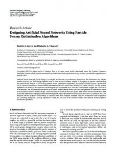
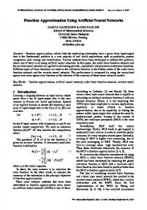
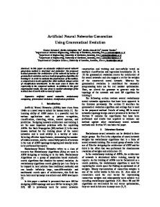
Figure 1: The remaining error plotted as function of the sizes of the two hidden modules. node, and the possible ways to treat the existing weights. Ideas taken from cascaded-correlation [7], and growing cell-structures [10] were tried, which increased the learning speed compared with random initializations [5]. To give an impression of the results of this relatively simple algorithm we show some experiments we did with the ‘What/Where’ problem [22], where 9 different 3x3 patterns are presented on all 9 possible positions in a 5x5 grid, giving a total of 81 different input/output patterns. The network has to learn which pattern is presented where. Strictly speaking, this problem can be learned without hidden layer. When however a hidden module is present, the problem becomes more difficult to solve (due to interference of the two tasks). Then, better results are obtained when the hidden module is divided among the two separate tasks giving a separate hidden module for each task. The original experiment was neurological in nature: it tried to explain why there are separate neurological pathways in the brain concerned with the detection of objects and the position of those objects. Fig. 1 gives the average sum-squared error of ten repetitions of training 300 cycli using backpropagation with momentum for several sizes of the two hidden modules. Table 1 gives the consecutive module sizes of our algorithm for the two subnetworks. It is easy to see that our algorithm follows the optimal path, and learns the task, which demonstrates that it is correctly determining the module where the next node should be added. More experiments are described in [5].
5
Table 1: Results of the what/where experiment. Step
0
1
2
3
4
5
6
7
…
19
What
1
1
1
1
1
2
2
3
…
15
Where 1
2
3
4
5
5
6
6
…
6
5 Initiating the “Baldwin effect” Baldwin was the first to recognize the impact of adaptive behavior of individuals on evolution [1]. He showed that ‘Lamarckism’ was not necessary to explain that learned behaviour seems to propagate through the genes of successive generations, but that instead, the inherited character was the ability to learn, with a profitable effect on the fitness of the individual. The same effect can be used in evolutionary computation applied to neural networks. When learning is part of the fitness evaluation when searching for a good set of weights for a given architecture, a significant speed-up and final quality of solution can be achieved [2, 15]. Also when using evolutionary computation to optimize architectures, learning can increase performance [3,12], but sofar these attempts have been restricted to learning weights. With the algorithm presented in this paper, it will be possible to optimize modular artificial neural network architectures, ‘implementing’ the Baldwin effect not just by learning weights, but by adapting the modular structure itself as well. However, as already observed by Whitley et al. [23], the Baldwin effect usually results in better solutions than the Lamarckian approach, but it also takes more time. Therefore, we are currently implementing this scheme on a parallel supercomputer (CM5), to try some real world problems.
6 Conclusions and further work Looking at several recent studies in the area of neural network architecture optimization, our conclusion is that current computers are just beginning to be fast enough to test existing methods on really large problems. Recognizing the need for more scalable methods has resulted in several approaches using grammars. Moreover, effects known from biology that can increase the speed of artificial evolution are getting more and more attention. In order to cope with the increasing complexity of our world, fully understood methods with deterministic operations will in the future no longer have the needed strength. What might be called a messy approach will be better suited. Evolu-
6
tionary computation will perhaps continue to be the only search strategy able to generate the desired complexity.
7 References [1]
J.M. Baldwin; ‘A new factor in evolution.’ In: American Naturalist, 30, 441–451, 1896.
[2]
R.K. Belew; ‘When both individuals and populations search: adding simple learning to the genetic algorithm’. In: J.D. Schaffer (Ed.); Proceedings of the third International Conference on Genetic Algorithms, 34–41, Kaufmann, San Mateo, CA, 1989.
[3]
E.J.W. Boers and H. Kuiper; Biological Metaphors and the Design of Modular Artificial Neural Networks. MSc. Thesis, Leiden University, 1992.
[4]
E.J.W. Boers, H. Kuiper, B.L.M. Happel and I.G. Sprinkhuizen-Kuyper; ‘Designing modular artificial neural networks’. In: H.A. Wijshoff; Computing Science in The Netherlands: Proceedings (CSN’93), Ed.: H.A. Wijshoff, 87–96, Stichting Mathematisch Centrum, Amsterdam, 1993.
[5]
M.V. Borst; Local Structure Optimization in Evolutionairy Generated Neural Network Architectures. MSc. Thesis, Leiden University, 1994.
[6]
Y.L. Cun, J. Denker and S. Solla; ‘Optimal brain damage’. In: Advances in Neural Information Processing Systems, 2, 598–605, 1990.
[7]
S.E. Fahlman and C. Lebiere; ‘The Cascaded-Correlation Learning Architecture’. In: Advances in Neural Information Processing Systems, 2, 524-532, 1990.
[8]
D.B. Fogel; ‘An introduction to simulated evolutionary optimization’. In: IEEE Transactions on Neural Networks, 5, 3–14, 1994.
[9]
M. Fréan; ‘The Upstart algorithm: a method for constructing and training feedforward neural networks’. In: Neural Computations, 2, 198– 209, 1990.
[10] B. Fritzke; ‘Growing cell structures - A self-organizing network for unsupervised and supervised Learning. TR-93-026, 1993. [11] F. Gruau; Neural Network Synthesis Using Cellular Encoding and the Genetic Algorithm. PhD. Thesis, l’Ecole Normale Supérieure de Lyon, 1994.
7
[12] F. Gruau and D. Whitley; ‘Adding learning to the cellular development of neural networks: evolution and the Baldwin effect’. In: Evolutionary Computation, 1, 213–233, 1993. [13] B.L.M. Happel and J.M.J. Murre; ‘Design and evolution of modular neural network architectures’. In: Neural Networks, 7, 985–1004, 1994. [14] S.A. Harp, T. Samad and A. Guha; ‘Towards the genetic synthesis of neural networks’. In: J.D. Schaffer (Ed.); Proceedings of the third International Conference on Genetic Algorithms (ICGA), 360–369, Kaufmann, San Mateo, CA, 1989.. [15] G.E. Hinton and S.J. Nowlan; ‘How learning can guide evolution’. In: Complex Systems, 1, 495–502, 1987 [16] H. Kitano; ‘Designing neural network using genetic algorithm with graph generation system’. Complex Systems, 4, 461–476, 1990. [17] M. Marchand, M. Golea and P. Ruján; ‘A convergence theorem for sequential learning in two-layer perceptrons’. In: Europhysics Letters, 11, 487–492, 1990. [18] M. Mezard and J.-P. Nadal; ‘Learning in feedforward layered networks: the Tiling algorithm’. In: Journal of Physics A, 22, 2191–2204, 1989. [19] E. Mjolsness; ‘Bayesian interference on visual grammars by neural nets that optimize’. Technical Report YALEU-DCS-TR-854, Yale University, 1990. [20] M. Mozer and P. Smolensky; ‘Skeletonization: a technique for trimming the fat from a network via relevance assessment’. In: Advances in Neural Information Processing Systems, 1, 107–115, 1989. [21] C.W. Omlin and C.L. Giles; Pruning recurrent neural networks for improved generalization performance. Revised Technical Report No. 93-6, Computer Science Department, Rensselaer Polytechnic Institute, Troy, N.Y., 1993. [22] J.G. Rueckl, K.R. Cave and S.M. Kosslyn; ‘Why are “what” and “where” processed by separate cortical visual systems? A computational investigation’. In: Journal of Cognitive Neuroscience, 1, 171– 186, 1989. [23] D. Whitley, V.S. Gordon and K. Mathias; ‘Lamarckian evolution, the Baldwin effect and function optimization’. In: Y Davidor, H.-P. Schwefel and R. Männer (Eds.); Lecture Notes in Computer Science, 866, 6–15, Springer-Verlag, 1994.
8