Evolving Dispatching Rules for solving the ... - Human Competitive

Evolving Dispatching Rules for solving the Flexible Job-Shop Problem Nhu Binh HO

Joc Cing TAY*

Evolutionary and Complex Systems Lab School of Computer Engineering Nanyang Technological University, Singapore 639798 [email protected]

Evolutionary and Complex Systems Lab School of Computer Engineering Nanyang Technological University, Singapore 639798 [email protected]

Abstract- We solve the Flexible Job-Shop Problem (FJSP) by using dispatching rules discovered through Genetic Programming (GP). While Simple Priority Rules (SPR) have been widely applied in practice, their efficacy remains poor due to lack of a global view. Composite Dispatching Rules (CDR) have been shown to be more effective as they are constructed through human experience. In this paper, we employ suitable parameter and operator spaces for evolving CDRs using GP, with an aim towards greater scalability and flexibility. Experimental results show that CDRs generated by our GP framework outperforms the SPRs and CDRs selected from literature in 74% to 85% of FJSP problem instances.

The classical JSP and FJSP have been solved by many local search methods, such as Simulated Annealing [4], Tabu Search [5][9][10], or Genetic Algorithms [11]-[14]. These previous results show that these techniques can find optimal or near optimal results. However, a major disadvantage is their huge computational cost, particularly when the problem size increases. In practice, dispatching rules have been applied to overcome these costs faced by the former [15]-[17]. Although dispatching rules are unable to fare better than the local search methods, they are the more frequently applied heuristics due to their ease of implementation and their low time complexity. Whenever a machine is available, a priority-based dispatching rule inspects the waiting jobs and selects the job with the highest priority to be processed next. Recently, the introduction of composite dispatching rules (CDR) have been increasingly investigated by the some researchers [18][19], but typically only for classical JSPs. These rules are the heuristic combination of single dispatching rules that aim to inherit the advantages of the former. The results show that, with careful combination, the composite dispatching rules do perform better than the single ones in the quality of schedules. In this paper, we investigate the potential use of GP for evolving effective composite dispatching rules for solving the FJSP with recirculation, with the objective of minimizing total tardiness. The ultimate purpose is to find rules that better human-made dispatching rules in solving the same problem. We intend to use them to solve the FJSP and the other similar problems without any additional algorithmic improvements. The remainder of this paper is organized as follows. Section 2 gives the formal definition of the FJSP with recirculation. Section 3 reviews recent related works for solving the JSP and FJSP using dispatching rules and a overview of GP. Section 4 describes our proposed GP framework for evolving CDRs while Section 5 analyzes the performance results of the CDRs obtained with GP. Finally, Section 6 gives some concluding remarks and directions for future work.*

1 Introduction In today’s highly competitive marketplace, a high level of delivery performance has become necessary to satisfy customers. Due to market trends, product orders of low volume – high variety types have been increasing in demand. Hoitomt et al. [1] mentions that these products comprise between 50 to 75 % of all manufactured components, thereby making schedule optimization an indispensable step in the overall manufacturing process. The Job-Shop Scheduling Problem (JSP) is one of the most popular manufacturing optimization model in practice [2]. It has attracted many researchers due to its wide applicability and inherent difficulty [3]-[6]. It is also well known that the JSP is NP-hard [7], hence general, deterministic methods of search are in general inefficient. The nxm classical JSP involves n jobs and m machines. Each job is to be processed on each machine in a predefined sequence, and each machine processing only one job at a time. In practice, the shop-floor setup typically consists of multiple copies of the most critical machines so that bottlenecks due to long operations or busy machines can be reduced. Therefore, an operation may be processed on more than one machine having the same function. This leads to a more complex problem known as the Flexible Job-Shop Scheduling Problem (FJSP). The extension involves two decisions; assignment of an operation to an appropriate machine and sequencing the operations on each machine. In addition, for complex manufacturing systems, a job can typically visit a machine more than once (known as recirculation). These three features of the FJSP significantly increase the complexity of finding optimal solutions [8].

2 Problem Definition Similar to the classical JSP, solving the FJSP requires the optimal assignment of each operation of each job to a *

corresponding author.

machine with known starting and completion times. However, the task is more challenging than the classical one because it requires a proper selection of a machine from a set of machines to process each operation of each job. Furthermore, if a job is allowed to recirculate, this will significantly increase the complexity of the system [20]. The FJSP with recirculation is formulated as follows: • Let J = {Ji}1≤i≤n, indexed i, be a set of n jobs to be scheduled. • Each job Ji consists of a predetermined sequence of operations Gi = {Oi,j}1≤j≤O(i) where Oi,j denotes operation j of Ji and O(i) is the total number of operations of job Ji. • Let M = {Mk}1≤k≤m, indexed k, be a set of m machines. • Each machine can process only one operation at a time. • Each operation Oi,j can be processed without interruption on one of a set of machines F(Oi,j) ⊆ M. Therefore, we denote by Oi,j,k to be operation j of Ji that is processed on machine Mk and pi,j,k be its processing time on machine Mk. • Recirculation occurs when a job can visit a machine more than once. Formally, this implies

∃i , j1 , j2 : F (Oi , j1 ) ∩ F (Oi , j2 ) ≠ ∅

• Let Ci and di be the completion time and the due date of the job Ji, respectively. The tardiness of this job is calculated by the following formula: Ti = max {0, Ci - di} • The objective function T of this problem is to find a schedule that minimizes the sum of tardiness of all jobs (total tardiness problem): n

n

i =1

i =1

T = ∑ Ti = ∑ max ( 0, Ci − di )

If F(Oi,j) is the set of machines that operation Oi,j can be processed on, then the FJSP is further classified into two sub-problems as follows: • Total FJSP (T-FJSP): each operation can be processed on any one machine of set M: F(Oi.j) = M. • Partial FJSP (P-FJSP): each operation can be processed on one machine of subset of M: F(Oi,,j) ⊂ M. Total tardiness is one of the major objectives in production scheduling. A job that is late may penalize the company’s reputation and reduce customer satisfaction. Hence, keeping the due dates of jobs under control is one of the most important tasks faced by companies [19]. In this paper, we shall assume that • All machines are available at time 0. • Each job has its own release date and due date. • The order of operations for each job is predefined and cannot be modified.

3 Previous Works Dispatching rules have received much attention from researchers over the past decades [15]-[17]. In general, whenever a machine is freed, a job with the highest priority in the queue is selected to be processed on a machine or work center. A comprehensive survey on dispatching rules is by Panwalkar and Wafik [15] and Blackstone et al. [16]. Depending on the specification of each rule, it can be classified [15] into: • Simple Priority Rules • CDRs • Weighted Priority Indexes • Heuristic Scheduling Rules Simple Priority Rules (SPR) are usually based on a single objective function. They usually involve only one model parameter, such as processing time, due date, number of operations or arrival time. The Shortest Processing Time (SPT) is an example of a SPR. It orders the jobs on the queue in the order of increasing processing times. When a machine is freed, the next job with the shortest time in the queue will be removed for processing. SPT has been found to be the best rule for minimizing the mean flowtime and number of tardy jobs [17]. The Earliest Due Date (EDD) is another example of a SPR where the next job to be processed is the one with the earliest due date. Unfortunately, no SPR performs well across every performance measure such as tardiness or flow time [21]. To overcome this limitation, CDRs have been studied to combine good features from such SPRs. There are two kinds of CDRs presented in literature; the first type involves deploying a select number of SPRs at different machines or work centers. Each machine or work center employs a single rule. When a job enters a specific machine or work center, it is processed by the SPR that is predetermined for that machine or work center. For instance, Barman [21] applied three different SPRs to solve the flow shop problem corresponding to three work centers. Experimental results show that it obtains better results than a single SPR that is common to all three machines. However, this approach may not be suitable for a shop floor with large number of machines or work centers; and the best independent use of single SPRs is difficult to predetermine. Furthermore, it still has the limitation of a localized view. The second type involves applying the composition of several SPRs (otherwise known as a CDR) to evaluate the priorities of jobs on the queue [17]. The latter type is executed similarly to SPRs; when a machine is free, this CDR evaluates the queue and then selects the job with the highest priority. For example, Oliver and Chandrasekharan [17] present five CDRs for solving the JSP. Their results indicate that CDRs are more effective compared to individual SPRs. CDRs inherit the simplicity of SPRs while achieving some scalability as the number of machines increase. Furthermore, if well designed, CDRs can solve realistic problems with multiple objectives [8]. However, the challenge is to find a good combination of SPRs to apply to all machines or work centers.

Weighted priority index rules are the linear combination of SPRs described above with computed weights [18][19]. Depending on specific business domains, the importance of a job determines it’s weight. For instance, considering n jobs with different weights w, where weight wi is assigned to job Ji. The sum of the weighted tardiness as the objective function is given as follows: n

n

i =1

i =1

T = ∑ wiTi = ∑ wi × max ( 0, Ci − di )

In this paper, the weighted priority rules are not considered as they are a generalization of our current formulation of total tardiness where we have assumed instead that all jobs have the same weight (see Section 2). Heuristic rules are rules that depend on the configuration of the system. These rules are usually used together with previous rules, such as SPRs, CDRs or weighted priority index rules. For instance, the heuristic rule may use the expertise of human experience, such as inserting an operation of a job into an idle time slot by visual inspection of a schedule [15]. The results from recent researchers [17][21] show that CDRs outperform individual SPRs in minimizing the performance of shop floor. In this work, we focus our attention on finding a computational method to build effective CDRs; one that is based on the composition of fundamental measures rather than on the algebraic combination of SPRs. However, this may be difficult to enumerate manually due to the large parameter and operator space, hence we employ a GP framework. Genetic programming (GP) [22] belongs to a family of evolutionary computation methods. It is based on the Darwinian principle of reproduction and survival of the fittest. Given a set of functions and terminals and an initial population of randomly generated syntax trees (representing programs), the programs are evolved through genetic recombination and natural selection. GP has been applied to many different problems; from classical tasks, such as function fitting or pattern recognition, to non-trivial tasks that are competitive with significant human endeavours such as designing electrical circuits [23] or antennas [24]. The most important feature that makes GP different from the canonical GA is it’s ability to vary the logical structure and size of evolved computer programs dynamically. It can therefore solve more challenging problems that have eluded the canonical GA due to the latter’s requirement of a fixed-length chromosome. However, GP has rarely been applied to manufacturing optimization; this is due to the direct permutation property of scheduling where jobs and/or machines can be simply reordered (in the case of JSP) to obtain better results. For instance, the chromosomes presented in [10]-[14] have fixed lengths, which can be evolved easily by direct permutation. On the other hand, GP uses a tree-based encoding with dynamic length; making it difficult to encode the JSP (for that matter, a FJSP) into a tree-based chromosome. Unlike previous approaches [17]-[19], [21] where a predefined set of SPRs were combined in advance by human experience, we apply GP to find

superior constructions of CDRs which composed of fundamental terminals (see Table I). These discovered rules are then used to solve the FJSP directly; the advantage being, the obtained CDRs can solve the FJSPs in shorter computational time as compared to genetic algorithms [10]-[14]. Recently, GP has been used to solve the classical one machine tardiness problem [25]. However, the results of for this specific problem with a smaller number of parameters cannot not be applied to solve general scheduling problems, such as the FJSP. In the next Section, we will present a GP framework with an important number of parameters suited for the FJSP. The obtained results described in Section 5 are simple and meaningful. We believe that this GP framework could be used to solve other problems such as the flexible flow shop or open shop.

4 Design of the GP Framework In GP, an individual (ie, computer program) is composed of terminals and functions. Therefore, when applying GP to solve a specific problem, they should be well designed to satisfy the requirements of the current problem. After evaluating many parameters related to the FJSP, the terminal set and the function set that are used in our algorithm are described as follows. 4.1 Terminal set In job-shop scheduling, there are many parameters that can effect the quality of results; potentially, all of them can be considered to comprise a dispatching rule. However, in order to create a short and meaningful dispatching rule, only a small and sufficient number of parameters should be evaluated properly. They also help to reduce the search space and improve the efficiency of the algorithm. Based upon the dispatching rules involving due dates in [15]-[17] and our experimental works, the terminal set proposed in this study is given in Table I. TABLE I TERMINAL SET Terminal ReleaseDate DueDate ProcessingTime CurrentTime RemainingTime numOfOperations avgTotalProcTime

Meaning Release date of a job (RD) Due date of a job (DD) Processing time of each operation (PT) Current time (CT) Remaining processing time of each job (RT) Number of operations of each job (nOps) Average total processing time of each job (aTPT)

In Table I, CurrentTime represents the time when a particular machine is free and starts to select a job to process on its queue. RemainingTime corresponds to the elapsed time for the current job to finish. Some previous dispatching rules use total processing time of each job as one of their parameters. However, in FJSP, an operation of each job can be processed on a set of machines (see

Section 2). We normalize the average processing time of each operation with the following formula: ∑ pi , j ,k pi , j =

n ( F ( Oi , j ))

n( F (Oi , j ))

where pi,j,k stands for processing time of operation Oi,j on machine Mk and n(F(Oi,j) represents number of machines that can process Oi,j. 4.2 Function set Similar to other applications of GP [22]-[24] for solving optimization problems, we use four basic operators: addition, subtraction, multiplication, and division for creating our CDR. Furthermore, we employ a well-known Automatically Defined Function (ADF) (proposed by Koza [26]). The ADF is sub-tree which can be used as a function in the main tree. The size of the ADF is varied in the same manner as the main tree. It enables GP to define useful and reusable subroutines dynamically during its run. The results from [26] indicate that GP using ADF outperforms GP without ADF in solving the same optimization problem. The more parameters that are used in ADF, the more changes will be needed for GP to evolve good subroutines. However, it can lead to a higher number of generations. We limit the ADF used in our approach to two parameters. The operators used in the ADF are also the four basic operators mentioned above. The operators of the function set in our approach are given in Table II. TABLE II FUNCTION SET Function + − ∗ / ADF(x1, x2)

Meaning Addition Subtraction Multiplication Division Automatically Defined Function

4.3 Fitness function The obtained results from each generation of GP are a set of computer programs modeled as trees. As mentioned in Section 2, the objective in our study is to minimize the total tardiness of the FJSPs. Therefore, we propose a method to form a CDR from the tree-based result of GP. This CDR is then combined with the least waiting time rule [13] to evaluate the total tardiness of the FJSPs. The FJSP is solved by applying two processes in succession. The first one finds a suitable machine to process each operation, and the second finds a proper order of operations on each machine’s queue. These two processes are described in detail as follows. To find a suitable machine (routing) to process an operation Oi,j, we apply the least waiting time rule [13] on the set of setting machines that can process Oi,j. This rule is intended to reduce the workloads of the machines by balancing operations to be assigned. It is calculated by summing up the processing times of all the subsequent operations in the waiting list plus the remaining processing time on each machine and the processing time

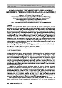
of Oi,j. Therefore, it depends on the total time this operation has to wait to be processed in the worst case, not relying only on its own processing time. In determining the proper order of operations on the queue of a particular machine, we use the CDR generated by GP. When a machine is freed, the generated rule is applied directly to the set of operations that are waiting on the queue of the machine. The operation with the highest priority is then selected to be processed on the machine. Figure 1 below gives an example of a dispatching rule tree generated by GP: progn defun

x1 x2

ADF

values /

∗ x1

values

−

x2 DD

+ −

CT DD

RD

ADF PT

nOps

Fig. 1. Example of a GP tree with defined functions and terminals

Figure 1 shows the overall structure of the generated tree that gives a possible CDR. The left child of progn shows the function-defining branch (containing the defun). In this case, the ADF function is defined by: ADF(x1,x2)=x1∗x2. The right child gives the resultproducing branch. This CDR therefore represents the following formula: ( DD − CT )

( DD − RD ) + ADF ( PR, nOps)

Since ADF(x1,x2)=x1∗x2, we obtain: ( DD − CT )

( DD − RD ) + ( PR ∗ nOps )

Any tree in the genomic population of GP that contains our defined functions and terminals can be interpreted as a CDR in the same way.

5 Experimental results This Section reports and analyses the empirical results for evaluating the efficiency of our proposed algorithms. The framework was implemented using C++ running on a 2 GHz PC with 512 MB RAM. 5.1 Test Case Generation Various experiments were conducted. We categorized these experiments into three classes: T-FJSP, P-FJSP with

50% of flexibility (P-FJSP-50), and P-FJSP with 20% of flexibility (P-FJSP-20). The P-FJSP with c% of flexibility means that less than c% of all machines are selected to process an operation. Number of jobs and number of machines range from 10 to 200 and 5 to 15, respectively. Processing time of each operation was drawn out of U((number of machines)/2, (number of machines)×2) (U represents the uniform distribution function). In practice, an operation can be processed on any of a group of machines that constitute a work center. Deviation of these processing times is ideally zero or usually small. Therefore, in our test cases, we set the maximum deviation between two operations to be 5 unit times. The release date of each job depends on the number of jobs in a particular test case. If the number of jobs is larger than 50, the release date is drawn out of U[0,40], else it is taken from U[0,20]. Baker [27] proposed a formula to estimate the due date of a job using the TWK-method: ni

di = ri + c × ∑ pij

TABLE III CHOICE OF PARAMETER VALUES Parameters

Value

Population Size Number of Generations Creation Type Maximum depth for creation Maximum depth for crossover

100 200 Ramped half and half 7 17

Crossover Probability

100%

Swap Mutation Probability

3%

Shrink Mutation Probability

3%

Number of best rules copy to new generation

5

5.3 Data Analysis The best five dispatching rules that were selected from 5 runs times of GP on the training set are given in Table IV; where possible, they were simplified algebraically. Each GP run took 12.81 hours to complete the training set.

j =1

where ri and di denote release and due dates of job i respectively. pij presents the processing time of operation Oij, and c denotes the tightness factor of the due date. The higher the value of c, the looser is the job’s due date. We adapt this formula to generate due dates of jobs with a replacement of the parameter piq with piq . Depending on the tightness of the due date, we separate the samples of each class T-FJSP, P-FJSP-50, or P-FJSP-20 into tight, moderate, or loose due date corresponding to values of c = 1.2, 1.5, and 2. We also generate mixed samples where each sample contains 34% jobs with tight due dates, 33% of jobs with moderate due dates, and the remaining ones with loose due dates. Specifically, the class T-FJSP holds 9 samples of tight due date, 9 samples of moderate due date, 9 samples of loose due date, and 9 samples of mix due date. Similarly for PFJSP-50 and P-FJSP-20, with 36 samples each. Each training set contains three classes of 108 FJSP problems with different number of jobs, machines and different tightness of jobs. Another five validation sets of similar compositions were generated. The average results of the five validation sets were then reported. 5.2 Parameter setting Through experimentation, the set of suitable parameter values used in our GP framework is listed in Table III. We implemented Ramped half and half to generate the initial population of GP. This method was proposed by Koza [22] and it has been widely used by previous researchers. It divides the initial population into two parts. Half of the initial population contains the random generated trees with maximum depth (in this experiment, this value is 7). The remaining part of the initial population contains the random generated trees with depth values ranging from one to the maximum depth. In order to keep the best trees that may be destroyed by GP’s operators, we sorted the current population and copied five of them to the next generation.

TABLE IV GP GENERATED DISPATCHING RULES Rule

Expression

Rule_1

aTPT ∗ (CT +RD + PT − 3 )+ (CT ∗ PT + RD + nOps) − (nOps ∗ PT + 2PT+CT+1)

Rule_2

( PT+ CT+ RD + 2 ) ∗ (RT+ PT + aTPT)

Rule_3

CT ∗ aTPT + 5nOps + 3RD

Rule_4

DD ∗ (RD + aTPT + RT + PT)

Rule_5

( aTPT + PT) ∗ (CT + RD) + (DD - RD)

In order to compare the efficiency of the evolved rules to the human-made rules presented in literature, some of frequently used single and composite dispatching rules were selected [16]: • FIFO (First In First Out). • SPT (Shortest Processing Time). • EDD (Earliest Due Date). • MDD (Modified Due Date) = max{CT+PTi, DDi} [18]. • SL (Slack Time) = DDi – CT – RTi [17]. The selected rules are also combined with the least waiting time rule [13] to evaluate the total tardiness of the FJSPs (see Section 4.3). Table V below compares the results of Rule_1 and the five selected dispatching rules for solving T-FJSP with different due date tightness.

TABLE V COMPARING PERFORMANCE OF DISPATCHING RULES ON T-FJSP Rule

Tight

Moderate

Loose

FIFO SL SPT MDD EDD Rule_1

56698.04 57035.16 45019.78 41747.31 30884.33 30868.89

54494.69 50716.69 43101.13 38426.49 28594.82 28588.07

50991.18 40837.24 39024.53 33294.87 24827.18 24813.33

Mix 54037.56 47317.84 42762.09 38362.49 29111.04 28156.51

Results from Table V show that the FIFO rule performs poorly in comparison with the others. This is because the due dates of jobs are ignored by FIFO, and therefore the rule does not focus on minimizing total tardiness. The composite dispatching rule SL can obtain slightly better results than FIFO but its results are still poor in comparison to the remaining rules. Table V indicates that MDD outperforms SL. From the definition of MDD and SL described above, we observe that although these two composite rules contain similar parameters (DD and CT), the gap between the results of the two rules are quite large due to different algebraic combinations of the parameters. This emphasizes that the functions that combine the rules can significantly affect the results. Blackstone et al. [16] mentioned that the SPT seems to be the best rule when the problem does specify due dates or have very tight due dates for a classical job shop. When the problem specifies loose or moderate due dates then EDD seems to be the best. However, the results presented in Table V indicate the contrary, that EDD outperforms SPT for all classes of tight due-dates when solving the FJSP. EDD is the best rule among five rules selected from literature (FIFO, SPT, EDD, MDD, SL) in solving T-FJSP. This could be explained by the flexibility feature of FJSPs where an operation can be processed on one of a group of machines. When a FJSP specifies tight due dates, each job in this problem still has alternative routes to take through the system, not just one route as in the classical JSP. Therefore, if the job on the queue is selected by EDD, it has more likely to finish on time. Although the other rules such as SL or MDD also contain the parameter - due date (DD), EDD obtains almost 50% better results than these rules. This again demonstrates that if an ineffective composite dispatching rule is applied to specific problems, it may achieve worse results than the single ones. The best performing rule in Table V is the generated rule - Rule_1. This rule performs slightly better than EDD in solving problems with tight or moderate due dates, but for the loose and mix due date loads, it is better than EDD. Table VI and Table VII below compares the effectiveness of the generated rule - Rule_1 to the five dispatching rules from literature for solving the FJSP problems with different tightness on machine assignment. The values in two tables show that when the shop is less flexible, there are more tardy jobs. The observed quality of the rules in solving these FJSP problems remain similar to results in Table V. The EDD still outperforms the other

dispatching rules in solving the P-FJSP with 50% and 20% flexibility. Rule_1 remains the best for solving the same problems. Table VI and Table VII also demonstrates that when the shop is less flexible, Rule_1 is still much better than EDD on loose and mix due date problems. TABLE VI COMPARING PERFORMANCE OF DISPATCHING RULES ON P-FJSP WITH 50% FLEXIBILITY Rule

Tight

Moderate

Loose

FIFO SL SPT MDD EDD Rule_1

59984.31 59812.00 48778.44 45497.78 33276.33 33233.16

58119.93 53131.51 46326.53 41904.98 30891.76 30901.20

54183.93 43076.04 42702.47 36446.64 27110.93 27035.47

Mix 57233.27 49119.18 45437.40 40933.71 31068.89 30090.89

TABLE VII COMPARING PERFORMANCE OF DISPATCHING RULES ON P-FJSP WITH 20% FLEXIBILITY Rule

Tight

Moderate

Loose

FIFO SL SPT MDD EDD Rule_1

63848.09 61611.89 52274.91 49144.64 36797.33 36358.47

61366.56 54097.24 50422.31 45729.60 34308.91 33795.56

56797.36 42499.18 44913.31 38990.09 29692.22 29156.11

Mix 61628.31 51239.93 49603.13 45431.42 35264.09 33746.71

Table VIII summarizes and sorts the results for average tardiness when using Rule_1 and for other rules in solving the FJSP to minimize total tardiness. Note that the value given in each column is the average tardiness value for 180 different instances. TABLE VIII COMPARING RULE_1 WITH OTHER SINGLE AND COMPOSITE RULES

Rule

T-FJSP

FIFO SL SPT MDD EDD Rule_1

54055.37 48976.73 42476.88 37957.79 28354.34 28144.20

P-FJSP with 50% flexibility 57380.36 51284.68 45811.21 41195.78 30586.98 30315.18

P-FJSP with 20% flexibility 60910.08 52362.06 49303.42 44823.94 34015.64 33264.21

In general, the FIFO obtains the worst results among the five selected rules from literature. The EDD emerges to be the best among the selected rules. Its performance is found to be significantly better than the SPT in all kinds of due date tightness. This finding is quite interesting because the existing literature notes that the SPT is an efficient rule under highly loaded job-shop conditions [17]. The best performing rule is the evolved rule Rule_1. The values in bold-faced identify the instances where Rule_1 is observed to be fare better than the remaining ones. When the flexibility of the shop is tighter, Rule_1 still achieves better results than EDD. We now compare the other generated rules against the most effective rule (EDD) among the selected rules from

literature. Table IX shows the proportion of instances that the EDD had fared poorer and better than the five generated rules. The improvement by using the generated rules was significant overall. They obtained better results for 74% to 85% of problem instances when compared to EDD. In addition, Rule_1 outperformed the other rules in terms of the proportion of instances that it solved. It can be observed that at least 85% of instances solved by Rule_1 fared better than those solved by the most effective human-made rule EDD. In this sense, it can be concluded that the evolved rules produced by our GP framework is very competitive with the human-made rules selected from literature. TABLE IX COMPARING FIVE EVOLVED DISPATCHING RULES WITH THE EDD RULE Rule Rule_1 Rule_2 Rule_3 Rule_4 Rule_5

Percentage of instances EDD was worse 85.19% 81.48% 77.78% 75.00% 74.07%

Percentage of instances EDD was better 14.81% 18.72% 22.22% 25.00% 25.93%

In order to understand why these evolved rules are effective in solving the FJSP to minimize total tardiness, we now take a closer look at the combination of their parameters. While single rules consider only one parameter of the shop, the evolved rules employ almost all the important parameters. However, the combination of these parameters plays an essential role to the success of the rule. For instance, the composite rules SL and MDD combine the parameter DD with other parameters CT, PT, and RT but they fail to get better results than the EDD with just one parameter DD (see Table VIII). The parameters aTPT and RD could be important for solving the problem. They are present in all the rules and contribute mainly to change the priority of one operation to be selected in a queue. For example, Rule_2 in Table IV was constructed with two terms. The first term operates in favor of release date RD and processing time PT while the second term runs in favor of average total processing time aTPT and remaining time RT. When the release date of a job is small, this means that the job is released early, the first term produces small results. Similarly, when the remaining time of the job is small, the second term produces a small result. Both parameters help to decrease the value of the ratio and assign a high priority to the job. It is well known that the SPT rule is effective in minimizing the number of tardy jobs [17]. Two terms of this rule also contains PT and aTPT that are in favor of the SPT. Therefore, they also contribute to improve the efficacy of the rule.

6 Conclusion and Future Works In this paper, a GP-based approach for discovering effective composite dispatching rules for solving the FJSP

has been presented and analyzed. CDRs have been studied widely by previous researchers [15]-[17]. However, all of them were constructed based on the experience of a human scheduler. We employ a GP-framework to generate a CDR based on fundamental terminals that can effectively solve the FJSP (together with a machine assignment rule) to minimize total tardiness. Five composite dispatching rules were generated by GP over a large training set. These rules are based on the combination of parameters such as processing time, release date, due date, current time, number of operations, and average total processing time of each job using basic arithmetical operators. Extensive simulations have been carried out to evaluate the performance of the five evolved rules over varying degrees of problem flexibilities and due date tightness. Five other popular rules selected from literature were also evaluated as performance benchmarks. It was found that EDD is significantly better than the other rules from literature. However, all the generated rules found by GP outperformed the EDD for 74% to 85% of the problem instances. Several possible extensions of this study can be developed. Similar to other applications of GP where the parameters are sensitive, denser terminal sets and more varied ADRs should be investigated to improve the generated rules. The approach of this study can be applied to find the efficient composite dispatching rules for other similar problems, such as a flow shop or the classical job shop. The rules evolved from this GP framework are still quite complex to simplify. Therefore, a simplification algebraic simplification tool could be used to make the formula more meaningful. Consideration could even be given to including the number of parameters used as a measure for minimization. Finally, the redundant parameters in each evolved rule can be examined further to get better results.

Acknowledgments This research was funded in part by Technological University and CEI Manufacturing Limited Company, Singapore.

Nanyang Contract

Bibliography [1] D. J. Hoitomt, P. B. Luh, and K. R. Pattipati, ”Practical Approach to Job-Shop Scheduling Problems,” IEEE Transactions on Robotics and Automation, vol. 9(1), pp. 1-13., 1993. [2] A.S.Jain and S.Meeran, “Deterministic job-shop scheduling: Past, present and future,” European Journal of Operation Research, vol. 113(2), pp. 390434, 1998. [3] J.Carlier and E.Pinson, “An algorithm for solving the Job-Shop problem,” Management Science, vol. 35(2) pp. 164-176, 1999. [4] M. Kolonko, “Some New Results on Simulated Annealing Applied to the Job Shop Scheduling Problem,” European Journal of Operational Research, vol. 113, pp. 123-136, 1999.

[5] E. Nowicki and C. Smutnicki, “A Fast Taboo Search Algorithm for the Job Shop Problem,” Management Science, vol. 42(6), pp. 797-813, 1996. [6] T.Yamada, R.Nakano, “A fusion of crossover and local search,” Proc. IEEE International Conference on Industrial Technology, pp. 426–430, 1996. [7] M.R. Garey, D.S. Johnson, R. Sethi, “The complexity of flow shop and job-shop scheduling,” Mathematics of Operations Research, vol. 1(2), pp. 117-129, 1996. [8] M. Pinedo. and X. Chao, Operations scheduling with applications in manufacturing and services, MCGraw-Hill , 1999, Chaper 3. [9] P. Brandimarte, “Routing and scheduling in a flexible job shop by tabu search,” Annals of Operations Research, vol. 22, pp. 158-183, 1993. [10] M. Mastrolilli, L.M. Gambardella, "Effective Neighborhood Functions for the Flexible Job Shop Problem", Journal of Scheduling, vol. 3(1), pp. 3-20, 2000. [11] I. Kacem, S. Hammadi, and P. Borne, “Approach by localization and multiobjective evolutionary optimization for flexible job-shop scheduling problems,” IEEE Transactions on Systems, Man and Cybernetics, vol. 32(1), pp. 1-13, 2002. [12] I. Kacem., S. Hammadi, P. Borne, “Paretooptimality approach for flexible job-shop scheduling problems: hybridization of evolutionary algorithms and fuzzy logic,” Mathematics and Computers in Simulation, vol. 60, pp. 245-276, 2002. [13] N. B. Ho and J. C. Tay, “GENACE: An Efficient Cultural Algorithm for Solving the Flexible JobShop Problem,” Proc. the Congress on Evolutionary Computation CEC2004, pp. 1759-1766, 2004. [14] J. C. Tay and D. Wibowo, “An Effective Chromosome Representation for Evolving Flexible Job-Shop Schedules,” Proc. Genetic and Evolutionary Computation GECCO2004, pp. 210221, 2004. [15] S. Panwalkar and I. Wafik, “A Survey of Scheduling Rules,” Operations Research, vol. 25(1), pp. 45-61, 1977. [16] J.H. Blackstone, D.T. Phillips, G.L. Hogg, "A stateof-the-art survey of dispatching rules for manufacturing job shop operations", International Journal of Production Research, vol. 20(1), 1982. [17] H. Oliver and R. Chandrasekharan, “Efficient dispatching rules for scheduling in a job shop,” International Journal of Production Economics, vol. 48(1), pp. 87-105, 1997. [18] J.K. John, L. Xiaoming, "A Weighted Modified Due Date Rule for Sequencing to Minimize Weighted Tardiness", Journal of Scheduling, vol. 7(4), pp. 261-276, 2004. [19] M. S. Jayamohan and C. Rajendran, "Development and analysis of cost-based dispatching rules for job shop scheduling," European Journal of Operational Research, vol. 157(2), pp. 307-321, 2004. [20] M. Pinedo, Scheduling theory, algorithms, and systems, Prentice Hall, 2002, Chaper 2.

[21] S. Barman, "Simple Priority Rule Combinations: An Approach To Improve Both Flow Time And Tardiness," International Journal of Production Research, vol. 35(10),pp. 2857-2870, 1997. [22] J. Koza, Genetic Programming: on the programming of computers by means of natural selection, Cambrige, MA: MIT Press, 1992. [23] J.R. Koza, F.H. Bennett III, D. Andre, M.A. Keane, F. Dunlap, “Automated Synthesis of Analog Electrical Circuits by Means of Genetic Programming,” IEEE Transactions on Evolutionary Computation, vol. 1(2), pp.109-128, 1997. [24] J. D. Lohn, G. S. Hornby, D. S. Linden, “An Evolved Antenna for Deployment on NASA's Space Technology 5 Mission,” Proc. Genetic Programming Theory Practice 2004 Workshop (GPTP-2004), 2004. [25] C. Dimopoulos, A.M.S. Zalzala, "Investigating the use of genetic programming for a classic onemachine scheduling problem," Advances in Engineering Software, vol. 32 (6), pp. 489-498, 2001. [26] J. Koza, Genetic Programming II, Automatic Discovery of Resuable Programs, MIT Press, 1994, Chapter 4. [27] K.R. Baker, "Sequencing Rules and Due-date Assignments in Job Shop," Management Science, vol. 30, pp. 1093-1104, 1984.