Evolving Evolution Programs: Genetic Programming and L-Systems Christian Jacob Lehrstuhl für Programmiersprachen Martensstr. 3, Universität Erlangen-Nürnberg D-91058 Erlangen, Germany
[email protected] http://www2.informatik.uni-erlangen.de/IMMD-II/Persons/jacob ABSTRACT Parallel rewrite systems in the form of string based L-systems are used for modeling and visualizing growth processes of artificial plants. It is demonstrated how to use evolutionary algorithms for inferring L-systems encoding structures with characteristic properties. We describe our Mathematica based genetic programming system Evolvica, present an L-system encoding via expressions, and explain how to generate, modify and breed L-systems through simulated evolution techniques. Extensions of genetic programming operators and expression generation methods strongly relying on templates and pattern matching are shown by example.
1.
Lindenmayer (1990)), as we will demonstrate in this paper. D0L-systems (D0 means deterministic with no context) are the simplest type of L-systems. Formally, a D0L-system can be defined as a triple G = ( Σ, P, α ) where Σ = { σ 1, …, σ n } is an alphabet, α , the initial start word * commonly referred to as the axiom, is an element of Σ , the set of all finite words over the alphabet Σ . The structure * preserving D0L-mapping P : Σ → Σ is defined by a set of contextfree productions or rewrite rules σ → P ( σ ) for each σ ∈ Σ . Let us consider the following L-system which models a simple growth process: Σ = { f, sprout, stalk, pd, leaf, bloom } α
: p1 : p2 : p3 :
α
The formation of structures in nature is always the result of complex growth processes. One idea of evolutionary biology is that structure formation can be interpreted as the execution of »programs« or rewrite rules. These programs are highly parametrized where the parameters are set by the environment in which development and interaction processes take place. Generally, rewriting has proved to be a useful technique for defining complex objects by successively replacing parts of simple initial objects using a set of rewrite rules or productions. In the scope of this article we will focus on a special type of character based rewrite systems, commonly termed L-systems (Lindenmayer systems), which are used in theoretical biology for describing and simulating natural growth processes, Lindenmayer (1968). All letters in a given word are replaced in parallel and simultaneously. This feature makes L-systems especially suitable for describing fractal structures, cell divisions in multicellular organisms (Jacob (1994), Jacob (1995)), or flowering stages of herbaceous plants (Prusinkiewicz and
D k
sprout ( 4 ) → f stalk(2) [ pd(60) leaf(0) sprout(3) ] bloom(0) sprout(t0) → f f stalk(t-1)
Applying the rules p 1 , p 2 , and p 3 first to the start word α , and then repeatedly to the resulting expressions generates the following sequence of words:
Modeling growth processes by L-systems
Di
sprout ( 4 )
d
: :
sprout ( 4 )
2
:
f f f stalk(1) [ pd(60) leaf(0) sprout(4) ] bloom(0)
3
:
f f f f f stalk(0) [ pd(60) leaf(0)
P ( α) P ( α) P ( α)
f stalk(2) [ pd(60) leaf(0) sprout(3) ] bloom(0)
f stalk(2) [ pd(60) leaf(0) sprout(3) ] bloom(0) ] bloom(0)
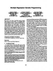
... In the example L-system given above production p 3 encodes elongation of a stalk segment, and p 1 describes part of a stalk and a bloom, together with another sprout segment enclosing a leaf and branching from the main axis. In order to translate these expressions into spatial structures resembling three-dimensional plant architectures we have to define a geometrical interpretation of the strings. More specifically, we will use a variant of the so-called turtle geometry, the basic idea of which is to interpret some of the alphabet symbols Σ as commands to maneuver a virtual drawing tool, known as a turtle, in 3D space. The turtle can thus change its position and orientation and draw lines or graphical elements while being moved around in three dimensions. Figure 1 shows an animation sequence for the turtle interpretation of a more complex parametrized L-
ll
i F
M k
404
(9)
(10)
Initial start word: sprout(4) Sprout developing leaves and flower: p 1 : sprout(4)
→ f stalk(2) [ pd(60) leaf(0) ] pu(20) [ pu(25) sprout(0) ] [ pd(60) leaf(0) ] pd(20) [ pu(25) sprout(2) ] f stalk(1) bloom(0)
Riping sprout: p 2 : sprout(t < 4) → sprout(t+1)
Figure 1
(7)
(6)
(5)
(8)
Stalk elongation: p 3 : stalk(t > 0)
→ f f stalk(t-1)
Changing leaf sizes: p4 p5 p6 p7
: : : :
leaf(t) leaf(t > 7) Leaf(t) Leaf(t < 2)
→ → → →
leaf(t + 1.5) Leaf(7) Leaf(t - 1.5) leaf(0)
Growing bloom: p 8 : bloom(t) p 9 : bloom(7)
→ bloom(t + 1) → bloom(1)
L-system modeling of growth processes for plantlike geometrical structures
system describing growth sequences of sprouts, leaves and blooms of an artificial flower. Besides the elementary turtle commands this D0L-system encodes macros for generating graphical representations of the leaves, blooms and stalks. All the non-italic terms (f, pu, pd) represent commands to move the turtle (f: forward, b: backward) and change the drawing tool´s orientation by rotation around its longitudinal, lateral, and vertical axes (rl/rr: roll left/right, pu/pd: pitch up/down, yl/yr: yaw left/right), thus translating a one-
dimensional string into a 3D-object resembling a plant. In order to be able to generate branching structures a kind of stacking mechanism for the turtle´s position and orientation is necessary. For each string of the form s 1 [ s 2 ] s 3 the strings s 1 , s 2 , and s 3 are interpreted in sequence, however, before starting the interpretation of s 2 the current turtle position and orientation are pushed on a stack, so that, having finished interpreting s 2 , the turtle is reset to its prior coordinates and orientation.
AXIOM,
(1)
1.
LSystem[
2. 3.
AXIOM[sprout[4]], LRULES[ LRule[LEFT[], PRED[ sprout[4] ], RIGHT[], SUCC[SEQ[SEQ[f],SEQ[stalk[2]], STACK[PD[60],leaf[0]], ...,
LRULES],
(1)
SEQ, SEQ[f],SEQ[stalk[1]], bloom[0]]]], LRule[LEFT[], PRED[ sprout[t r → s with l, p, r and s denoting the left context, predecessor, right context and successor, respectively. The symbols "" separate context and predecessor strings. Thus each rule can be represented by an expression of the form LRule[ LEFT[ l ], PRED[ p ], RIGHT[ r ], SUCC[ s ] ].
Accordingly, an L-system with its axiom and rule set is encoded by an expression of the form LSystem[
AXIOM, LRULES[
LRule] ],
where we use a pattern notation with F denoting a term of the form F[...], and F representing a non-empty sequence of F expressions. So our example L-system of section 1 would be represented as follows: LSystem[AXIOM[sprout[4]], LRULES[ LRule[LEFT[],PRED[sprout[4]],RIGHT[], SUCC[f,stalk[3], STACK[pd[60],...],bloom[0]]], LRule[LEFT[],PRED[sprout[t0]],RIGHT[], SUCC[f,f,stalk[t-1]]],
where L-system bracketing of the form [s] is now represented as STACK[s].
2.2
Stochastic generation of L-system codings
One of the main differences of our GP approach to the GP paradigm introduced by Koza (1992) is the use of high-level building blocks for expression generation as well as modification. Instead of just defining a set of function symbols together with their arities, each expression from a template pool, as depicted in figure 2, serves as a possibly partial description of a genotype, encoding an L-system in our case. Each of these templates (marked with 1., 2., 3., ...) is associated with a set of attributes like, e.g., predicates constraining the set of subexpressions that can be plugged in. Thus the encoded L-system productions are restricted to contextfree forms (4., LEFT[], RIGHT[]) with their left-hand sides (4., PRED) constrained to sprout[i], with i replaced by an integer number from the interval, say, [0,4] (5.), and their right-hand sides (4., SUCC) defined either as a sequence (SEQ) of expressions (6., 7. and 8.) or a bracketed expression sequence (6., STACK). Each expression is constructed from a start pattern (here: LSystem[ AXIOM, LRULES]) by recursively inserting matching expressions from the expression pool until all pattern blanks – marked by – have been replaced by according subexpressions. Of course, one has to take care that this construction loop eventually ends. Some further remarks should be made about the enco-
ding scheme of figure 2. The templates basically describe the D0L-system of figure 1. However, the additional SEQ pattern within the first LRule expression (3.) enables the generation system to create rule variations by inserting new expression sequences, i.e. one or more expressions of the form SEQ[...]. Accordingly, the L-system encoding might be enhanced by additional rules by replacing the LRule pattern with a (possibly empty) sequence of LRule[...] expressions. Each sequence of expressions is constructed via alternative templates (7. and 8.), where SEQ[ [a|b|c]] denotes an arbitrary sequence of expressions taken from the set {a,b,c} as, e.g., SEQ[a,a,c,b] or SEQ[c,c,c,a,b,a] with the sequence length restricted to, say, between 4 and 6. Whenever there are several templates matching one pattern the expressions are selected with probabilities proportional to their weights (see the bracketed numbers right from the expressions in figure 2, serving as fitness values for the templates). The pattern matching is not unique for the SEQ pattern (6.) for which there are two matching templates (7. and 8.), a recursive (SEQ[.... SEQ]) and non-recursive version which will be selected with a probability of 0.8, thus implicitly restricting the nesting of expressions.
2.3
Variations on L-system expressions
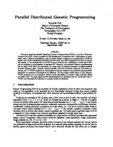
The following is a small collection of operators used for generating variations on arbitrary expressions (figure 3). As with the expression generating operators the basic idea is to use again templates for controling which subexpressions should be in the scope of each operator: • Mutation replaces a randomly selected subexpression by an expression – with the same head expression – generated from the template pool. • Crossover is a recombination operator between two or more expressions. Subexpressions with the same head are selected within the expressions and interchanged. • Deletion erases expression arguments whenever this is possible according to restrictions of the number of arguments for the selected expression. • Duplication inserts a copy of a randomly selected argument as an additional subexpression. • Permutation interchanges the sequence of arguements of an expression. These operators are defined for general expressions and are not especially tailored to L-system encodings. Subexpressions are chosen according to operator specific selection schemes based on pattern matching mechanisms. Thus it is, e.g., possible to restrict recombinations to subexpressions with head SUCC, i.e. expressions of the form SUCC[...], which allows to interchange right-hand sides of L-system productions, or permute only LRule expressions thus changing the ordering of rules. With a set of templates defined for each operator the effects of genetic operators can be constrained in a problem specific way which turns out to be important especially in the case of interactive »breeding« of expressi-
Operator pool ω dupl
Population of expressions
f a f g c a b
ω repro
f hc g f c b bd d ge h f b bc d g e h a b dg g cb d
ω decaps
ω cross
ω mut
Ω
ω del
ω perm
ω encaps
(2)
∆Ω
(1) s:
Structure-selection templates
... ω mut
f
g e
g [ x:
h
a b dg
h Length ( x ) > 1
]
g
c b
d
∆ = g [ x:
g
]
(3)
f
(4)
Length ( x ) > 1
e
h
g a b d g (5) c b d g
t:
ω mut
a b d s´:
g c
c
g
(6) b
f e
h
b g c b
Figure 3
t´:
(7) g d
Example of expression variations by using genetic operators with pattern matching capabilities
ons as in the case of evolution-based L-system inference. Figure 3 shows the general scheme for the application of genetic operators, exemplified by the mutation operator, and how these operators extensively use pattern matching techniques. (1) An expression s to be modified by a genetic operator is selected from the population of expressions. (2) An operator – attributed each with a weighting selection probability – is chosen from an operator pool Ω. (3) The operator to be applied, the mutation operator for this example, then selects an expression template ∆ from its operator specific pattern pool ∆Ω. (4) According to the ∆-template matching subexpressions of s are identified. (5) Among the set of those matching subexpressions one is chosen at random. (6) Finally, the operator specific modifications are applied. (7) In the case of the mutation operator this means that the subexpression is replaced by a newly generated expression with the same head.
3.
Breeding artificial flowers
With all the ingredients described above we are now able to demonstrate how plant like structures with specific characteristics can be developed with the help of L-system evolution. Suppose we want to breed flowers similar to those introduced in section 1. However, suppose we want to breed species which spread out far in x-, y- and z-direction and carry as many leaves and blooms as possible. The fitness function used for the following example evolution takes just this criterion into account and is defined as follows: M
fitness ( plant ) =
∑ ∆xi ⋅ ∆yi ⋅ ∆zi + 2 ⋅ Bi + Li i=0
∆x , ∆y , ∆z : extension of the geometric plant structure
in x-, y-, and z-dimension B : the number of blooms blossoming L : the number of leaves the plant carries M : the maximum number of L-system iterations The total fitness is computed as the sum of the plant´s extension, blooms, and leaves for each L-system iteration. This means that fitness does not only depend on how the plant flourishes at a certain growth stage but on the whole structure generation process from an initial sprout to a fullgrown plant. In the following simple example we start with a small population of six L-system genomes each generated with the templates of figure 2. A maximum number of M = 6 Lsystem iterations is used. Figure 4 shows three stages of a typical evolution sequence over eight generations. The indi-
viduals are selected proportional to their fitness. Table 1 lists the set of operators and operator-specific templates that were used for evolutionary L-system synthesis. Table 1 Genetic operators, their application probabilities, and according sets of templates with template selection probabilities Operator
Prob.
Selection templates
TProb.
Mutation
0.35
LRule SEQ STACK
0.2 0.4 0.4
Crossover
0.35
LRule SEQ STACK
0.2 0.4 0.4
Deletion
0.1
LRULES[ | l > 1] SEQ[ | l > 1] STACK[ | l > 1]
Duplication
0.1
- ditto
- ditto
Permutation
0.1
- ditto
- ditto
0.2 0.4 0.4
Even with a very limited number of individuals, as in our example, it turns out that the evolution system is able to create rather complex plantlike structures even within only a few generations. Figure 4 shows such a typical evolution run with an exponential increase of the best fitness values ranging from below 40 at the beginning to above 2500 in generation 8. From initially rather small individuals widespread plants evolve carrying bunches of blooms and leaves. On the phenotypical level it is striking that even in the very first generations (Gen. 2) the expressed plantlike structures exhibit a large range of divesity although all Lsystem encodings are just variants of the basic genotype template of figure 2. Those templates basically ensure, to a certain degree, that plantlike geometrical structures arise whereas the constrained composition of alternative patterns results in different morphogenetic characteristics of the same species or of a totally different species emerging (see, e.g., individuals 4 and 6 of generation 8). Some of the generated individuals have a very low fitness (gen. 2, indiv. 5,6) carrying no or only a few leaves. However, there are also individuals possessing the characteristic branching structure of the basic plant (figure 1) while trying to meet the fitness criterion by growing an increasing number of blossoming branches. While at the beginning those branches are rather short carrying only a few blooms, finally long branches prevail in generation 5 where bunches of blooms and leaves appear on the bough segments. Fitness is increased by an order of magnitude up to values around 700. Further fitness improvement is achieved by elongating
the stalks as well as shortening the ripening periods. Thus it turns out that even with this very simple example we can observe effects found in natural evolution periods of plant species as well. The rudimentary phylogenetic tree of figure 5 might serve as a demonstration. Over seven generations we can show the phenotypical stages of evolution for the best plant up to the final (8th) generation. Initially, there is a plant with three main branches with the leftmost carrying no leaves or blooms. Its descendants in generations 3 and 4 have grown in width and height and exhibit larger blooms. A decisive evolution step arises with generation 5; now all three main branches (with a smaller branch in the middle) carry a great number of blooms and leaves. In generation 6 even more branches have been created and the species is still enhancing its overall dimension which finally leads to the widespread, flourishing plant structure of generation 8. Figure 5 compares the evolved L-system encodings of generations 2 and 8, where it can be seen that the explained pheontypical effects are, of course, due to an increase of complexity within the genotypes. Generation 2: Axiom: sprout(4) sprout(4)
→
f stalk(2) [pd(60) leaf(0)] rr(90) [pd(20) sprout(3)] rr(90) stalk(0) rr(17) leaf(2) [pd(60) leaf(0)] rr(90) [pd(20) sprout(2)] f stalk(1) bloom(0)
sprout(t