Evolving Retrieval Algorithms with a Genetic ... - CiteSeerX

Evolving Retrieval Algorithms with a Genetic Programming Scheme James Theiler, Neal R. Harvey, Steven P. Brumby, John J. Szymanski, Steven Alferink, Simon Perkins, Reid Porter, and Jeffrey J. Bloch Space and Remote Sensing Sciences Group Los Alamos National Laboratory Los Alamos, New Mexico 87545 ABSTRACT The retrieval of scene properties (surface temperature, material type, vegetation health, etc.) from remotely sensed data is the ultimate goal of many earth observing satellites. The algorithms that have been developed for these retrievals are informed by physical models of how the raw data were generated. This includes models of radiation as emitted and/or reflected by the scene, propagated through the atmosphere, collected by the optics, detected by the sensor, and digitized by the electronics. To some extent, the retrieval is the inverse of this “forward” modeling problem. But in contrast to this forward modeling, the practical task of making inferences about the original scene usually requires some ad hoc assumptions, good physical intuition, and a healthy dose of trial and error. The standard MTI data processing pipeline will employ algorithms developed with this traditional approach. But we will discuss some preliminary research on the use of a genetic programming scheme to “evolve” retrieval algorithms. Such a scheme cannot compete with the physical intuition of a remote sensing scientist, but it may be able to automate some of the trial and error. In this scenario, a training set is used, which consists of multispectral image data and the associated “ground truth;” that is, a registered map of the desired retrieval quantity. The genetic programming scheme attempts to combine a core set of image processing primitives to produce an IDL (Interactive Data Language) program which estimates this retrieval quantity from the raw data. Keywords: Remote Sensing, Retrieval Algorithms, Image Processing, Genetic Algorithms, Genetic Programming

1. INTRODUCTION The importance of “end-to-end simulation” is often emphasized1–3 in the development and assessment of science retrieval algorithms. The front-end of an end-to-end simulation takes scene properties as given, and produces an accurate estimate of the imagery that is ultimately produced by the sensor. This involves direct physical modeling of the ambient radiation, the scene itself, the intervening atmospheric medium, and the sensor. The back-end of this simulation is the retrieval; it takes the (simulated) sensor data as input and produces as its output an estimate of the initial scene properties. Thus, the retrieval of scene properties from remotely sensed data is a problem of inversion. And the assessment of the retrieval algorithm is obtained by direct comparison of the scene properties that are provided in the original model (the “ground truth”) to the scene properties that are retrieved (“estimated truth”). The notion of retrieval as inversion appears in other applications as well. For example, in Refs. [4–6], a genetic algorithm was used to evolve a chain of morphological operators to reduce noise in video imagery for archival BBC footage. This was done by treating noise reduction as the inverse of noise corruption. Training sets were generated from an initial set of clean (“truth”) images and from the corrupted versions of those images which were generated by applying a known noise process. This approach is necessary as, in this application, there rarely (if ever!) exist uncorrupted and corrupted versions of the same data. After all, if you already have an clean version of the data, why bother attempting to “clean-up” a corrupted version? Work supported in part by the U.S. Departments of Energy and Defense. Emails: {jt,harve,brumby,szymanski,salferink,s.perkins,rporter,jbloch}@lanl.gov.

To appear in Proc SPIE 3753 (1999)

1

A generic retrieval provides a useful starting point, but an optimized retrieval is optimal only for a specific system. The normalized difference vegetation index (NDVI) produces a fair first cut at a vegetation map and is broadly applicable to a number of sensors, but for a specific sensor the best ratio of band differences will depend on which bands are available. Furthermore, a multi-spectral retrieval might be quite different from a hyper-spectral retrieval, not just in terms of different values for the parameters, but in terms of the functional form of the retrieval. The best retrieval can also depend on the properties of the scene. An algorithm that works well at detecting vegetation in the tropics might not recognize sagebrush in the desert. While the nature of the retrieval algorithm is informed by the physical principles that drive the forward model, the details are often “tweaked” to provide better agreement with whatever ground truth is available. The optimal backend retrieval depends, and often in a complicated way, on the details of the front-end simulation. For instance, the best choice of a smoothing kernel will probably depend on an instrument noise level. Depending on the complexity of the retrieval algorithm and the quality (and computational requirements) of the front-end simulation, this parameter adjustment can be a laborious process. And when the instrument flies, further tweaks may be called for. Most retrieval algorithms concentrate on either on spatial or spectral aspects of the image. As imagery becomes ever more finely resolved, in both the spatial and the spectral axes, the potential for a good spatio-spectral retrieval is enhanced. But while physical principles might indicate that a spatio-spectral retrieval is called for, it is difficult to know how best to combine the features of both, and in practice such combinations are ad hoc. Here too is an opportunity for automated retrieval design.

1.1. Obtaining ground truth The need for ground truth in machine-learning approaches is an important, sometimes debilitating, obstacle. For remote sensing retrievals, in particular, the collection of real ground truth data can be very expensive. One way around this is to use forward models to produce artifical data. In this case, the ground truth is part of the model and is known with complete accuracy and reliability. For instance Borel7 used a first-principles nonlinear spectral mixing model8 of a leaf canopy over a soil surface to produce multispectral signatures of vegetation for use in comparing various vegetation indices. The notion of vegetation index was extended in a follow-on paper by Gisler and Borel9 ; here a neural network was used to derive new vegetation indices based not on the forward model, but on the many training sets that the model could be called upon to generate. A second approach, sometimes called scaffolding10–13 or shaping,14,15 attempts to keep the human analyst “in the loop.” Using external information, context, and the unsurpassed pattern recognition capabilities of the retina and brain, the analyst identifies areas of real imagery as containing or not containing the feature of interest. The analyst needn’t identify every pixel, and the learning algorithm is rewarded/penalized for getting right/wrong only those pixels that the analyst identified. But once a candidate retrieval is identified, it is applied to all pixels. The analyst can critique the retrieval by identifying further pixels where the computer erred in its evaluation. On any iteration, the analyst need only identify a fraction of the total pixels – it is the analyst’s expertise, not patience, that is exercised.

2. GENETIC PROGRAMMING SCHEME A genetic algorithm (GA) is a scheme for searching a large solution space using a population of candidate solutions (chromosomes) which evolve by natural selection to perform some task, or achieve some goal, or solve some problem, or approximate some function, etc. The relative fitness of each chromosome is evaluated according to how well it performs its task, achieves its goal, solves its problem, etc. The least fit chromosomes are discarded, and those remaining serve as parents for a new generation of chromosomes. The new chromosomes are derived from the parent chromosomes either by small random changes (mutations) to the individual components of the chromosome (genes) or by combining the genes from two of the parents (recombination). As the population of chromosomes evolve, the individual chromosomes become increasingly fit for the task at hand. Mitchell’s book16 provides a recent overview of genetic algorithms. When the solution space is a space of computer programs, then the term genetic programming (GP) is usually applied. Koza17 provides an enthusiastic assessment of this approach. Like most machine-learning schemes, the goal is to generalize from examples. For our remote sensing applications, the examples are multiple “data planes” (corresponding, usually, to multiple spectral channels) of remote sensing imagery bundled with a “truth plane,” which contains the desired retrieval for every pixel. The goal is to evolve


2

Perl

IDL

Data

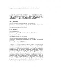
Figure 1. The genetic programming scheme is implemented in Perl and IDL. Evolution (mutation, recombination, and selection) is managed by a Perl script, while the computationally intensive image processing operations are performed in IDL. The high-bandwith communication with the data (and weight and truth) planes is done through the IDL program. The Perl script deals only with the chromosomes and their fitness scores, so the two-way unix pipe that connects the two processes is a low-bandwith connection.

a computer program (specifically, a multi-line program written in IDL18 which takes the data planes as input, and provides an estimate of the truth plane as output. In practice, six kinds of “planes” can be used: 1. Raw data planes contain the (real or simulated) sensor image data. 2. Optional pre-processed planes can be provided as if they were raw data planes; these allow the scientist to influence the GP scheme, by providing information that the GP is welcome (but not required) to exploit. 3. The truth plane provides the true value of the retrieval quantity for each pixel. The truth values can be discrete or continuous values, depending on the nature of the retrieval. Binary values may be appropriate for the identification of a specific feature (e.g., water or not water), while continuous values are appropriate for quantitative scene properties (e.g., water temperature). 4. The weight plane indicates which pixels of the truth plane to take seriously. If the truth is known for only a subset of the image, then this can be specified by setting the weight to zero at the unknown pixels. If the operator wants to convey increased importance or reliability for certain regions, this can also be encoded in the weight values. 5. Scratch planes (a.k.a. feature planes) contain images with intermediate processed results. These intermediate planes permit us to evolve more complex algorithms while maintaing our code as a simple string of image operators. 6. Answer planes are a specified subset of the data and scratch planes; these planes are combined to produce an estimated truth plane. In the simplest mode, there is a single answer plane, and at the end of the processing, it provides the estimated retrieval. The fitness of the candidate solution is given by the degree of agreement between this plane and the truth plane. If there are multiple answer planes, we presently use the best linear combination of the answer planes for our estimated truth. We are currently investigating the use of other classification schemes for the transformation of the answer planes into an estimate of truth. The genes in our chromosomes are single lines of IDL code that call an image operation subroutine. We use both spectral operators (various combinations of bands) and spatial operators (including a fairly extensive set of traditional/linear and non-linear operators – morphology: erode, dilate, close, open, etc., local averages: mean and median, local statistical measures: standard deviation, etc.). A gene reads one or more of the data and/or scratch planes, and then writes the result to one (or more, but usually just one) of the scratch planes. The data planes are never overwritten. The lines of IDL are executed in order, with no looping or back-tracking. After the last line has been executed, the answer planes are combined to produce an estimated truth plane. Fitness is based on the Euclidean distance between the estimated and final truth plane, with each pixel’s contribution to that distance proportional to its weight in the weight plane. The genetic algorithm is implemented in Perl, which communicates via a two-way pipe to an IDL process which does the image processing and fitness evaluation, as shown in Fig. 1. We have recently added a Java-based interface which permits the operator to specify more easily the values in the truth and weight planes interactively, thereby facilitating an iterative response to early results. Further details of our genetic programming scheme are presented elsewhere.19 To appear in Proc SPIE 3753 (1999)

3

3. RETRIEVALS Although most of the standard MTI data processing pipeline20 employs retrieval algorithms that have been developed directly from first principles modeling, many of these algorithms involve at least a few parameters: thresholds, coefficients of linear combinations, thresholds, etc. These parameters are generally fit to data that is already available, either from the calibration lab, from similar missions that have already flown, or from the simulation end of the endto-end model. These are simple examples, but they illustrate the separate roles of the scientist and the data-adaptive algorithm: the scientist decides on the form of the retrieval, the appropriate physical quantities, and the correct dimensional units; and the computer algorithm rapidly and systematically determines the fine details – in this case, the optimal values of the parameters. Our goal, in the subsequent examples, is to provide a more expansive role for the computer, to alleviate some of the more tedious aspects involved in deriving a retrieval algorithm, while still retaining the expertise and intuition of the scientist who “understands” the physics of the forward simulation.

3.1. Water Mask Water is ubiquitous in remote sensing imagery. Its properties are of interest their its own right; and because of its relative homogeneity compared to land surfaces, it is a useful backdrop in the retrieval of atmospheric properties. The water mask identifies which pixels in a registered multispectral image correspond to water. This is a binary mask, and is required as a first step for more sophisticated retrievals, such as water temperature and water quality retrieval. Water can be identified both by its spectral properties (low reflectance in the NIR and negative NDVI) and by its spatial properties (generally smooth and homogeneous, at least for larger bodies of water). The spatial properties in particular will depend on the details of the remote sensing platform: the ocean observed from low altitude on a windy day will have considerably more texture than Crater Lake as seen from a satellite. Further requirements may be placed on the spatial properties of the truth image. For instance, to reduce adjacency effects in the temperature retrieval, one may want a mask that only includes larger bodies of water and avoids the shoreline. For the MTI production pipeline, a water mask algorithm was developed by hand, combining in a physicallymotivated way both spatial and spectral operators. For the purpose of testing the Genetic Programming scheme, we took the production water mask as “truth” and attempted to produce an algorithm whose output would match this truth. The standard algorithm is a best-of-three vote among three simpler algorithms. Each of these simple algorithms was designed to capture some aspect or identify some specific type of water. The first cut captures some general characteristics of water, namely a low radiance in the NIR and a negative NDVI. The next two cuts were designed to include specific types of water. The second cut identifies large, uniform bodies of water by combining a spatial smoothness measure (standard deviation of radiance values in a kernel) with a negative NDVI. The third cut detects smaller bodies of water such as streams, ponds, and coastlines. To be classified as water under this cut, a pixel must have a low radiance in the NIR, a green/red ratio greater than one, and have a value less than the average of values in a surrounding kernel. Some preliminary results on the application of the GP scheme to this problem are described in Ref. [19].

3.2. Vegetation Water is water is water (well, more or less), but vegetation can be a jungle canopy in Guatemala, a corn field in Iowa, or a lone saguaro in Tombstone, Arizona. Nonetheless, nearly all vegetation exhibits a characteristic feature in the V/NIR (Visible and Near Infrared); it is dark in the red and bright in the near infrared. A number of indices that have been proposed for detecting vegetation in multispectral imagery are based on this red-edge feature (Borel7 reviews several of these, and compares their performance at identifying vegetation in an ab initio model). The most popular is the Normalized Difference Vegetation Index (NDVI), which is defined by NDVI =

ρnir − ρred ρnir + ρred

(1)

where ρν is the reflectance in band ν. To obtain a true reflectance requires atmospheric correction, but an often-used approximation employs the TOA radiance in place of reflectance in this formula.


4

(a)

(b)

(c)

(d)

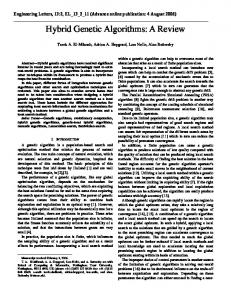
Figure 2. (a) Application of the NDVI index to the appropriate bands of 15-channel MAS data provides the “truth” plane which the Genetic Programming Scheme attempts to mimic. (b) Estimated truth from the best evolved algorithm is essentially identical to the original NDVI. (c) Estimated truth from an algorithm which did not include a normalized difference operator in the GP gene pool. (d) Best fit linear combination of data planes provides a simple estimate, against which the GP scheme can be compared. 3.2.1. NDVI as truth The task set for the Genetic Programming scheme was, as in the water mask case described previously, to produce an algorithm whose output would match an artifical “truth.” Unlike the water mask problem, however, the truth plane is not a binary mask but is the continuous values given by Eq. (1). Our data set was the first fifteen bands (0.523–1.914 µm) of radiance data from the MODIS (Moderate Resolution Imaging Spectrometer) Airborne Simulator (MAS21,22 ). For red, we used band 3 (0.679–0.721 µm), and for near-IR, we used an average of bands 5 and 6 (0.761–0.844 µm). Thus, the training set consisted of the 15-band MAS image data and the NDVI image “truth” shown in Fig. 2(a). The GP was then run on this training set. A population of fifty chromosomes was evolved, starting with random chromosomes, for five hundred generations. The best algorithm found by the GP at the end of the run was then applied to the 15-band MAS data set. The result is shown in Fig. 2(b). Subjectively, it can be seen that the resulting algorithm was able to produce an output that matched the “truth” image extremely well. To put some objective measure on this result, the root-mean-square difference between these images is about 0.2% of their full range. The algorithm found by the GP is described below. The 15 input data planes are labelled a, b, c, ..., o (despite the common nomenclature, these bands do not correspond with the 15 bands of MTI data). The algorithm used three scratch planes, labelled A, B, C. The answer planes included all the input data planes and the scratch planes, and the final answer was the best linear combination of these planes.


5

Scratch Band A B C

Coeff −0.0977 1.0226 0.0022

Data Band a f k

Coeff −0.0222 −0.0257 −0.0080

Data Band b g l

Coeff 0.0605 −0.0486 0.0408

Data Band c h m

Coeff 0.0495 −0.0237 0.0739

Data Band d i n

Coeff −0.0161 0.0198 0.0167

Data Band e j o

Coeff −0.0398 −0.0020 0.0135

Table 1. Coefficients for the linear combination of answer planes in the NDVI problem. The upper case values are scratch planes; the lower case are the raw data planes. The dominant coefficient is for scratch plane B, which is associated with the normalized difference operator.

Scratch Band A B C

Coeff 0.97667 0.15197 0.66169

Data Band a f k

Coeff 0.45914 0.02302 −0.37967

Data Band b g l

Coeff 0.21151 −0.02723 −0.17836

Data Band c h m

Coeff 0.15564 −0.01355 0.07275

Data Band d i n

Coeff 0.09135 0.05015 0.03766

Data Band e j o

Coeff 0.02601 −0.04464 0.02887

Table 2. Coefficients for the linear combination of answer planes in the NDVI problem for the case in which the gene pool did not contain a normalized difference operator.

Each line in the following algorithm represents an “active” gene in the best chromosome. The gene consists of an operator, input plane(s), output plane(s) and any other necessary parameters for the operator. A = divide_planes(a,b) B = norm_diff(c,e) C = sqrt(i) It can be seen that the resulting algorithm actually contains a normalized difference operator; in fact the input bands for the normalized difference operator are nearly the same as were used in the generation of this NDVI truth; these are band c (i.e., Red band 3) and band e (i.e., NIR band 5). Finally, from the coefficients for the linear combination of the answer planes (shown in Table 1), it can be seen that the dominant contribution to the final output image comes from the scratch band which is the output of the normalized difference operator (i.e., scratch plane B). We also ran the GP scheme using a set of genes that did not include the normalized difference operator. The algorithm that was found involved three separate band ratios. C = divide_planes(e,d) A = divide_planes(g,b) B = divide_planes(j,b) Looking at the coefficients of the back-end linear fit (Table ??), we see that the ratios C=e/d and A=g/b are the most important, and that these scratch planes are more important than any of the individual data bands. The error achieved by this algorithm was 1.6%. Finally, as a control experiment, we also found the best linear combination of the data planes. By eye, as seen in Fig. 2(d), the approximation is not too bad, but the error is about 8.8%. 3.2.2. “Bushy Tree” Identification The GP scheme was also given the task of identifying areas of an image containing what appear to be “bushy trees” from a 3-band Digital Orthoquad (DOQ) image provided by the United States Geological Survey (USGS). An example of an area of one of the data planes is shown in Fig. 3(a). To appear in Proc SPIE 3753 (1999)

6

(a)

(b)

(c)

Figure 3. (a) The “bushy trees” are readily seen by eye in the first channel (0.52–0.57 µm) of the raw data cube. (b) The hand-drawn truth plane indicates (in white) the pixels which the analyst confidently identifies as bushy trees. (c) The hand-drawn weight plane indicates (in white) which pixels to use as training data. Where the weight plane is white and the truth plane is black, the analyst has confidently identified as places where there are not bushy trees. Where the weight plane is black, the analyst has not made an identification one way or the other. (a) (b)

Figure 4. (a) Applying the best evolved algorithm to the data in “bushy trees problem” shown in Fig. 3(a) produces an estimate of the truth plane provided in Fig. 3(b). (b) Thresholding the estimated truth image in panel (a) shows that the bushy trees are indeed highlighted by this algorithm. Here, in contrast to the NDVI problem, we created a truth map by hand. This truth plane is shown in Fig 3(b). It can be seen that not all areas which contain “bushy trees” have been labelled: only generally, very obvious areas. The weight plane, shown in Fig. 3(c), indicates the confidence the analyst places in the truth values provided in the truth plane. Where the weight is zero, the truth data is meaningless, The GP scheme was then applied to this training set. The best algorithm found by the GP at the end of the run was then applied to the 3-band DOQ USGS data set. The result is shown in Fig. 4(a). It can be seen that the algorithm found by the GP scheme has been able to highlight the areas of the image in which there are the desired “bushy trees”. It should also be noted that the areas of the image containing the bushy trees which were not highlighted in the training set have been highlighted, as well as those areas in the training set. A thresholded image, as shown in Fig. 4(b) gives a better indication of the algorithm’s performance. The actual algorithm found by the GP scheme is shown below. The three input data planes are labelled a, b, c; the three scratch planes are labelled A, B C. The answer planes included all six planes. C = close_open(c,3,/circle) C = mean(C,7,/circle) A = divide_planes(C,b) To appear in Proc SPIE 3753 (1999)

7

Scratch Band A B C

Coefficient 0.8133 0.0000 1.3282

Data Band a b c

Coefficient 16.7700 -36.9398 9.4643

Table 3. Coefficients for the linear combination of answer planes in the bushy trees problem. (a)

(b)

(c)

Figure 5. (a) First band of an out-of-sample data set used for testing the bushy trees algorithm. (b) Estimated truth is obtained from the same algorithm (same operators, same parameters, and same linear combination at the back end) that was used in the training set. (c) Thresholded truth highlights where the bushy trees are predicted to be. The algorithm is applying a morphological close-opening with a 3 × 3 circular structuring element to the third data plane. This will smooth out highly localized fluctuations that are often found in otherwise flat or textureless areas such as the water. Then a local average, having a 7 × 7 circular window, is applied to this morphologically smoothed image. This will smooth out larger textures within the image. The ratio of this smoothed image and the unprocessed first data plane is then calculated. The coefficients for the linear combination of the answer planes are shown in Table 3. What can be seen here is that the unprocessed data planes provide a large contribution to the overall output and the scratch plane (B) not used by the algorithm, obviously makes no contribution at all. These coefficients indicate that the linear combination of the unprocessed data planes is the major contributor to the solution, and the contribution made by the (nonlinear) scratch planes is a small adjustment to that solution. But this small adjustment permits the solution to be much closer to the truth as provided by the analyst. It is, as in many approximation schemes, the last few percent which take the most effort to achieve. To estimate the out-of-sample performance of the algorithm found by the GP scheme, we applied it to data that was not part of the training set. This data was still part of the overall data set from which the training set was taken, but was from an entirely different region (i.e., no overlap between this data and training set). Fig. 5(a) shows the first channel of this out-of-sample data. We used the same algorithm (with the same linear coefficients) that was optimized for the training data, and applied it to the out-of-sample data. The result is shown in Fig. 5(b). The thresholded version of this image, seen in Fig. 5(c), shows that the correct areas of the image have been highlighted.

4. DISCUSSION A common problem of machine-learning schemes is that they try to solve the whole problem at once. There are, however, two human experts we are particularly keen to take advantage of. The first is the remote sensing scientist who understands the physical phenomenology of the forward model; the second is the technical analyst who has experience in interpreting imagery, and is skilled at identifying ground properties from these images. To appear in Proc SPIE 3753 (1999)

8

• An important role for the scientist is in determining which “data planes” should be used (usually, all of them!) and what preprocessed feature planes are expected to be useful. For instance, if it is an attribute of vegetation, then an NDVI plane can be added directly to the list of data planes. • The scientist is also called upon to provide the list of elementary operators that will be used to build up the full retrieval algorithms. While progress can be made by employing generic operators, the scientist has the opportunity to customize the nature of the solution by providing a set of image operators that are likely to be useful. • Ground truth campaigns are expensive, and although a necessary part of a remote sensing program, cannot be expected to provide the vast quantities of ground truth that pattern recognition software requires to do a good job. The technical analyst can often do a good job of estimating ground truth from subtle contextual cues that would be difficult to encode into an expert system. In particular, the analyst can critique the preliminary solutions provided by the GP scheme without identifying thousands of pixels worth of truth; instead, the analyst only identifies where the the automated scheme got it wrong. • Both the analyst and the scientist can provide a useful service in choosing an initial set of chromosomes. These can be chosen from “untweaked” versions of known retrieval algorithms, or from previously developed solutions to related problems.

ACKNOWLEDGEMENTS We are pleased to acknowledge Christoph Borel for numerous useful comments and discussions on some of the physical, mathematical, and computational issues involved in developing remote sensing retrievals, and for comments on this manuscript. We are also grateful to Melanie Mitchell for her assistance during the early stages of this project.

REFERENCES 1. B. W. Smith, C. C. Borel, W. B. Clodius, J. Theiler, B. Laubscher, and P. G. Weber, “End-to-end performance modeling of passive remote sensing systems,” in Infrared Imaging Systems: Design, Analysis, Modeling, and Testing VII, G. C. Holst, ed., Proc SPIE 2743, pp. 285–289, 1996. 2. P. G. Weber, C. C. Borel, W. B. Clodius, B. J. Cooke, and B. W. Smith, “Design considerations, modeling and analysis for the Multispectral Thermal Imager,” in Infrared Imaging Infrared Imaging Systems: Design, Analysis, Modeling, and Testing X, G. C. Holst, ed., Proc. SPIE 3701, 1999. 3. P. G. Weber, J. Theiler, B. W. Smith, S. P. Love, B. J. Cooke, W. B. Clodius, C. C. Borel, and S. C. Bender, “Measurement strategies for remote sensing applications,” in 1998 IEEE Aerospace Conference, Colorado March 6-13, 1999. 4. P. Kraft, N. R. Harvey, and S. Marshall, “Parallel genetic algorithms in the optimization of morphological filters: a general design tool,” J. Electronic Imaging 6, pp. 504–516, 1997. 5. N. R. Harvey and S. Marshall, “GA optimisation of spatio-temporal grey-scale soft morphological filters with applications in archive film restoration,” in Evolutionary Image Analysis, Signal Processing and Telecommunications (Proc. 1st European Workshop, EvoIASP’99 and EuroEcTel’99), R. Poli, H.-M. Voigt, S. Cagnoni, D. Corne, G. Smith, and T. Fogarty, eds., pp. 31–45, Springer-Verlag, (G¨ oteburg, Sweden), 1999. 6. This work is also described at the following website: http://www.spd.eee.strath.ac.uk/users/harve/bbc epsrc film dirt.html. 7. C. C. Borel, “Nonlinear spectral mixing theory to model multispectral signatures,” in Proc. 11th Thematic Conference on Geologic Remote Sensing, Vol. II, pp. 11–20, (Las Vegas, NV), 1996. 8. C. C. Borel and S. A. W. Gerstl, “Nonlinear spectral mixing models for vegetative and soil surfaces,” Remote Sensing of the Environment 47, pp. 403–416, 1994. 9. G. Gisler and C. Borel, “Neural network identifications of spectral signatures,” in Proc. 11th Thematic Conference on Geologic Remote Sensing, Vol. II, pp. 21–29, (Las Vegas, NV), 1996. 10. J. M. Daida, T. F. Bersano-Begey, S. J. Ross, and J. F. Vesecky, “Computer-assisted design of image classification algorithms: Dynamic and static fitness evaluations in a scaffolded genetic programming environment,” in Advances in Genetic Programming II, P. Angeline and K. Kinnear, eds., MIT Press, 1996.


9

11. J. M. Daida, J. D. Hommes, T. F. Bersano-Begey, S. J. Ross, and J. F. Vesecky, “Algorithm discovery using the genetic-programming paradigm: Extracting low-contrast curvilinear features from SAR images of arctic ice,” in Advances in Genetic Programming II, P. Angeline and K. Kinnear, eds., MIT Press, 1996. 12. J. M. Daida, T. F. Bersano-Begey, S. J. Ross, and J. F. Vesecky, “Evolving feature-extraction algorithms: Adapting genetic programming for image analysis in geoscience and remote sensing,” in Proc. 1996 International Geoscience and Remote Sensing Symposium: Remote Sensing for a Sustainable Future, IEEE Press, 1996. 13. J. M. Daida, R. G. Onstott, T. F. Bersano-Begey, S. J. Ross, and J. F. Vesecky, “Ice roughness classification and ERS SAR imagery of arctic sea ice: Evaluation of feature-extraction algorithms by genetic programming,” in Proc. 1996 International Geoscience and Remote Sensing Symposium: Remote Sensing for a Sustainable Future, IEEE Press, 1996. 14. M. Dorigo and M. Colombetti, Robot Shaping: An Experiment in Behaviour Engineering, MIT Press, Cambridge, Massachusetts, 1998. 15. S. Perkins and G. Hayes, “Evolving complex visual behaviors using genetic programming and shaping,” in Proc. 7th European Workshop on Learning Robots, (Edinburgh), 1998. 16. M. Mitchell, An Introduction to Genetic Algorithms, MIT Press, Cambridge, Massachusetts, 1996. 17. J. R. Koza, Genetic Programming: On the Programming of Computers by Means of Natural Selection, MIT Press, Cambridge, Massachusetts, 1992. 18. IDL (Interactive Data Language) is a commercial package for generic data and image processing, developed and marketed by Research Systems, Inc. (http://www.rsinc.com). 19. S. P. Brumby, J. Theiler, S. Perkins, N. Harvey, J. J. Szymanski, J. J. Bloch, and M. Mitchell, “Investigation of image feature extraction by a genetic algorithm,” in Applications and Science of Neural Networks, Fuzzy Systems, and Evolutionary Computation II, B. Bosacchi, D. B. Fogel, and J. C. Bezdek, eds., Proc SPIE 3812, 1999. 20. C. C. Borel, W. B. Clodius, A. B. Davis, B. W. Smith, J. J. Szymanski, J. Theiler, P. V. Villeneuve, and P. G. Weber, “MTI core science retrieval algorithms,” in Imaging Spectrometry V, M. R. Descour and S. S. Shen, eds., Proc SPIE 3753, 1999. 21. “The MODIS Airborne Simulator (MAS) is an airborne scanning spectrometer that acquires high spatial resolution imagery of cloud and surface features from its vantage point on-board a NASA ER-2 high-altitude research aircraft” (http://ltpwww.gsfc.nasa.gov/MODIS/MAS/Home.html). 22. M. D. King, W. P. Menzel, P. S. Grant, J. S. Myers, G. T. Arnold, S. E. Platnick, L. E. Gumley, S. C. Tsay, C. C. Moeller, M. Fitzgerald, K. S. Brown, and F. G. Osterwisch, “Airborne scanning spectrometer for remote sensing of cloud, aerosol, water vapor and surface properties,” J. Atmos. Oceanic Technol. 13, pp. 777–794, 1996.


10