scaling NE to large nets (i.e. tens of thousands of weights) ... efficients, to tasks that require very-large networks due to ..... positive; blue = large negative. (b) the ...
Evolving Large-Scale Neural Networks for Vision-Based Reinforcement Learning Jan Koutník
Giuseppe Cuccu
Jürgen Schmidhuber
Faustino Gomez
IDSIA, USI-SUPSI Galleria 2 Manno-Lugano, CH 6928
{hkou, giuse, juergen, tino}@idsia.ch ABSTRACT The idea of using evolutionary computation to train artificial neural networks, or neuroevolution (NE), for reinforcement learning (RL) tasks has now been around for over 20 years. However, as RL tasks become more challenging, the networks required become larger, as do their genomes. But, scaling NE to large nets (i.e. tens of thousands of weights) is infeasible using direct encodings that map genes one-toone to network components. In this paper, we scale-up our “compressed” network encoding where network weight matrices are represented indirectly as a set of Fourier-type coefficients, to tasks that require very-large networks due to the high-dimensionality of their input space. The approach is demonstrated successfully on two reinforcement learning tasks in which the control networks receive visual input: (1) a vision-based version of the octopus control task requiring networks with over 3 thousand weights, and (2) a version of the TORCS driving game where networks with over 1 million weights are evolved to drive a car around a track using video images from the driver’s perspective.
1.
INTRODUCTION
Neuroevolution (NE), has now been around for over 20 years. The main appeal of evolving neural networks instead of training them (e.g. backpropagation) is that it can potentially harness the universal function approximation capability of neural networks to solve reinforcement learning (RL) tasks without relying on noisy, nonstationary gradient information to perform temporal credit assignment. Early work in NE focused on evolving rather small networks (hundreds of weights) for RL benchmarks, and control problems with relatively few inputs/outputs. However, as RL tasks become more challenging, the networks required become larger, as do their genomes. The result is that scaling NE to large nets (i.e. tens of thousands of weights) is infeasible using a straightforward, direct encoding where genes map one-to-one to network components. Therefore, recent efforts have focused increasingly on indirect encodings [2, 3, 6, 7, 13] where relatively small genomes are transformed into networks of arbitrary size using a more complex mapping. In previous work [5, 8, 9, 14], we presented a new indirect encoding where network weight matrices are represented as Copyright is held by the author/owner(s). GECCO’13 Companion, July 6–10, 2013, Amsterdam, The Netherlands. ACM 978-1-4503-1964-5/13/07.
a set of coefficients that are transformed into weight values via an inverse Fourier-type transform, so that evolutionary search is conducted in the frequency-domain instead of weight space. The basic idea is that if nearby weights in the matrices are correlated, then this regularity can be encoded using fewer coefficients than weights, effectively reducing the search space dimensionality. For problems exhibiting a highdegree of redundancy, this “compressed” approach can result in an two orders of magnitude fewer free parameters and significant speedup [9]. With this encoding, networks with over 3000 weights were evolved to successfully control a high-dimensional version of the Octopus Arm task [16], by searching in the space of as few as 20 Fourier coefficients (164:1 compression ratio) [10]. In this paper, the approach is scaled up to two tasks that require networks with up to over 1 million weights, due to their use of high-dimensional, vision inputs: (1) a visual version of the aforementioned Octopus Arm task, and (2) a visual version of the TORCS race car driving environment. In the standard setup for TORCS, used now for several years in reinforcement learning competitions (e.g. [11]), a set of features describing the state of the car is provided to the driver. In the version used here, the controllers do not have access to these features, but instead must drive the car using only a stream of images from the driver’s perspective; no task-specific information is provided to the controller, and the controllers must compute the car velocity internally, via feedback (recurrent) connections, based on the history of observed images. To our knowledge this the first attempt to tackle TORCS using vision, and successfully evolve neural network controllers of this size. The next section describes the compressed network encoding in detail. Section 3 presents the experiments in the two test domains, which are discussed in section 4.
2.
COMPRESSED NETWORKS
Networks are encoded as a string or genome, g = {g1 , . . . , gk }, consisting of k substrings or chromosomes of real numbers representing DCT coefficients. The number of chromosomes is determined by the choice of network architecture, Ψ, and data structures used to decode the genome, specified by Ω={D1 , . . . , Dk }, where Dm , m = 1..k, is the dimensionality of the coefficient array P for chromosome m. The total number of coefficients, C = km=1 |gm | � N , is user-specified (for a compression ratio of N/C, where N is the number of weights in the network), and the coefficients are distributed evenly over the chromosomes. Which fre-
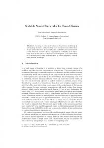
(a) Figure 1: Mapping the coefficients: The cuboidal array (top) is filled with the coefficients from chromosome g one simplex at a time, according to Algorithm 1, starting at the origin and moving to the opposite corner one simplex at a time. quencies should be included in the encoding is unknown. The approach taken here restricts the search space to bandlimited neural networks where the power spectrum of the weight matrices goes to zero above a specified limit frequency, cm ` , and chromosomes contain all frequencies up to m m cm ` , gm = (c0 , . . . , c` ). Figure 2 illustrates the procedure used to decode the genomes. In this example, a fully-recurrent neural network (on the right) is represented by k = 3 weight matrices, one for the input layer weights, one for the recurrent weights, and one for the bias weights. The weights in each matrix are generated from a different chromosome which is mapped into its own Dm -dimensional array with the same number of elements as its corresponding weight matrix; in the case shown, Ω={3, 3, 2}: 3D arrays for both the input and recurrent matrices, and a 2D array for the bias weights. Algorithm 1: Coefficient mapping(g, d) j ←0 K ← sort(diag(d) − I) P for i = 0 to |d| − 1 + |d| n=1 dn do l←0 P|d| si ← {e| k=1 eξj = i} while |si | > 0 do
ind[j] ← argmin e − K[l++ mod |d|] e∈si
si ← si \ ind[j ++] end end for i = 0 to |ind| do if i < |g| then coeff array[ind[i]] ← ci else coeff array[ind[i]] ← 0 end end In [9], the coefficient matrices were 2D, where the simplexes are just the secondary diagonals; starting in the topleft corner, each diagonal is filled alternately starting from its corners. However, if the task exhibits inherent structure that cannot be captured by low frequencies in a 2D layout,
(b)
Figure 3: Visual Octopus Arm. (a) The arm has to reach the goal (red dot) using a noisy visualization of the environment (b).
more compression can potentially be gained by organizing the coefficients in higher-dimensional arrays [10]. Each chromosome is mapped to its coefficient array according to Algorithm 1 (figure 1) which takes a list of array dimension sizes, d = (d1 , . . . , dDm ) and the chromosome, gm , to create a total ordering on the array elements, eξ1 ,...,ξDm . In the first loop, the array is partitioned into (Dm − 1)simplexes, where each simplex, si , contains only those elements e whose Cartesian coordinates, (ξ1 , . . . , ξDm ), sum to integer i. The elements of simplex si are ordered in the while loop according to their distance to the corner points, pi (i.e. those points having exactly one non-zero coordinate; see example points for a 3D-array in figure 1), which form the rows of matrix K = [p1 , . . . , pm ]T , sorted in descending order by their sole, non-zero dimension size. In each loop iteration, the coordinates of the element with the smallest Euclidean distance to the selected corner is appended to the list ind, and removed from si . The loop terminates when si is empty. After all of the simplexes have been traversed, the vector ind holds the ordered element coordinates. In the final loop, the array is filled with the coefficients from low to high frequency to the positions indicated by ind; the remaining positions are filled with zeroes. Finally, a Dm −dimensional inverse DCT transform is applied to the array to generate the weight values, which are mapped to their position in the corresponding 2D weight matrix. Once the k chromosomes have been transformed, the network is complete.
3.
EXPERIMENTS
Two vision-based control tasks were used to scale-up the compressed network encoding, the Visual Octopus Arm and Visual TORCS. All neural network controllers were evolved using the Cooperative Synapse NeuroEvolution (CoSyNE; [4]) algorithm.
3.1
Visual Octopus Arm
The octopus arm (see figure 3) consists of p compartments floating in a 2D water environment. Each compartment has a constant volume and contains three controllable muscles (dorsal, transverse and ventral). The state of a compartment is described by the x, y-coordinates of two of its corners plus their corresponding x and y velocities. Together with the arm base rotation, the arm has 8p + 2 state variables and
Fourier Space
Genome
Weight Space
Weight Matrices
|
Network
{z
g1
Inverse DCT
}|
Map
Map
=
{z
g2
}| {z
g3
}
|
{z Ω
|
}
{z
Ψ
}
Figure 2: Decoding the compressed networks. The figure shows the three step process involved in transforming a genome of frequency-domain coefficients into a recurrent neural network. First, the genome (left) is divided into k chromosomes, one for each of the weight matrices specified by the network architecture, Ψ. Each chromosome is mapped, by Algorithm 1, into a coefficient array of a dimensionality specified by Ω. In this example, an RNN with two inputs and four neurons is encoded as 8 coefficients. There are k = |Ω| = 3, chromosomes and Ω={3, 3, 2}. The second step is to apply the inverse DCT to each array to generate the weight values, which are mapped into the weight matrices in the last step. 3p + 2 control variables. In the vision-based version used here, the control network does not have access to the state variables. Instead it receives a noisy 32 × 32 pixel gray-scale image of the arm from a the perspective shown in figure 3(b). The goal of the task to reach a target position with the tip of the arm, from the starting position (arm hanging down) by contracting the 32 muscles appropriately at each 1s step of simulated time. Figure 3(a) shows the standard visualization the environment with the arm hanging down and two target positions shown in red. The idea of modifying an existing RL benchmark to use visual inputs dates back to the adaptive “broom balancer” of Tolat and Widrow [15], and more recently the vision-based mountain car in [1].
3.1.1
Setup
An evaluation consists of two trials, one with the target on the left, the other on the right, see figure 3. In each trial the target disappears after the first time-step, so that the network must remember which target is active throughout trial in order to solve the task. Having two target positions forces the controller to use the visual input instead of just outputting a fixed action sequence (i.e. open-loop control). The controllers were represented by fully-connected recurrent neural networks with 32 neurons, one for each muscle in the 10 compartment arm, for a total of 33,824 weights organized into 3 weight matrices. Twenty simulations were run with networks encoded using the following numbers of DCT coefficients: {10,20,40,80,160,320,640,1280,2560}. In all case the coefficients were mapped into 3 coefficient arrays using mapping Ω={4, 4, 2}: (1) a 4D array encodes the input weights from the 2D input image to the 2D array of neurons, so that each weight is correlated (a) with the weights of adjacent pixels for the same neuron, (b) with the weights for the same pixel for neurons that are adjacent in the 3 × 11 grid, and (c) with the weights from adjacent pixels connected to adjacent neurons; (2) a 4D array encodes the recurrent weights, again capturing three types of correla-
tion; (3) a 2D array encodes the hidden layer biases (see [10] for further discussion of higher-dimensional coefficient matrices). CoSyNE was used to evolve the coefficient genomes, with a population size of 128, a mutation rate of 0.8, and fitness computed as the average of the following score over the two trials: � � t d ,0 , (1) max 1 − T D where t is the number of time-steps before the arm touches the target, T is a number of time-steps in a trial, d is the final distance of the arm tip to the target and D is the initial distance of the arm tip to the goal. Each trial lasted for T = 200 time-steps.
3.1.2
Results
Figure 6 compare the performance of the various compressed encoding with the direct encoding in which evolution is conducted in 33,824-dimensional weight space. Using only 10 coefficients performs poorly but almost as well as the direct approach. With just 20 coefficient performance increases significantly, and after 40 coefficients, near optimal performance is achieved. For a video demo of the evolved behavior go to http://www.idsia.ch/~koutnik/images/octo pusVisual.mp4
3.2
Visual TORCS
The goal of the task is to evolve a recurrent neural network controller that can drive the car around a race track using only vision. The challenge for the controller is not only to interpret each static image as it is received, but also to retain information from previous images in order to compute the velocity of the car internally, via its feedback connections. The visual TORCS environment is based on TORCS version 1.3.1. The simulator had to be modified to provide images as input to the controllers. At each time-step during a network evaluation, an image rendered in OpenGL
(a)
(b)
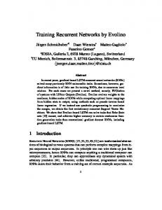
(c)
Figure 4: Visual TORCS environment. (a) The 1st-person perspective used as input to the RNN controllers (figure 5) to drive the car around the track. (b), a 3rd-person perspective of car. The controllers were evolved using a track (c) of length of 714.16m and road width of 10m, that consists of straight segments of length 50 and 100m and curves with radius of 25m. The car starts at the bottom (start line) and has to drive counter-clockwise. The track boundary has a width of 14m. is captured in the car code (C++), and passed via UDP to the client (Java), that contains the RNN controller. The client is wrapped into a Java class that provides methods for setting up the RNN weights, executing the evaluation, and returning the fitness score. These methods are called from Mathematica which is used to implement the compressed networks and the evolutionary search. The Java wrapper allows multiple controllers to be evaluated in parallel in different instances of the simulator via different UDP ports. This feature is critical for the experiments presented below since, unlike the non-vision-based TORCS, the costly image rendering, required for vision, cannot be disabled. The main drawback of the current implementation is that the images are captured from the screen buffer and, therefore, have to actually be rendered to the screen. Other tweaks to the original TORCS include changing the control frequency from 50 Hz to 5 Hz, and removing the “32-1-GO” waiting sequence from the beginning of each race. The image passed in the UDP is encoded as a message chunk with image prefix, followed by unsigned byte values of the image pixels. Each image is decomposed into the HSB color space and only the saturation (S) plane is passed in the message.
3.2.1
Setup
In each fitness evaluation, the car is placed at the starting line of the track shown in figure 4(c), and its mirror image, and a race is run for 25s of simulated time, resulting in a maximum of 125 time-steps at the 5Hz control frequency. At each control step (see figure 5), a raw 64 × 64 pixel image, taken from the driver’s perspective is split into three color planes (hue, saturation and brightness). The saturation plane is passed through Robert’s edge detector [12] and then fed into a Elman (recurrent) neural network (SRN) with 16 × 16 = 256 fully-interconnected neurons in the hidden layer, and 3 output neurons. The first two outputs, o1 , o2 , are averaged, (o1 + o2 )/2, to provide the steering signal, and the third neuron, o3 controls the brake and throttle
(−1 = full brake, 1 = full throttle). All neurons use sigmoidal activation functions. With this architecture, the networks have a total of 1,115, 139 weights, organized into 5 weight matrices. The weights are encoded indirectly by 200 DCT coefficients which are mapped into 5 coefficient arrays using mapping Ω={4, 4, 2, 3, 1} : (1) a 4D array encodes the input weights from the 2D input image to the 2D array of neurons in the hidden layer, so that each weight is correlated (a) with the weights of adjacent pixels for the same neuron, (b) with the weights for the same pixel for neurons that are adjacent in the 16 × 16 grid, and (c) with the weights from adjacent pixels connected to adjacent neurons; (2) a 4D array encodes the recurrent weights in the hidden layer, again capturing three types of correlations; (3) a 2D array encodes the hidden layer biases; (4) a 3D array encodes weights between the hidden layer and 3 output neurons; and (5) a 1D array with 3 elements encodes the output neuron biases. CoSyNE was used to evolve the coefficient genomes, with a population size of 64, a mutation rate of 0.8, and fitness being computed by: vmax 3m + − 100c , (2) 1000 5 where d is the distance along the track axis, vmax is maximum speed, m is the cumulative damage, and c is the sum of squares of the control signal differences, divided by the number of control variables, 3, and the number simulation control steps, T : f =d−
c=
3 T 1 XX [oi (t) − oi (t − 1)]2 . 3T i t
(3)
The maximum speed component in equation (2) forces the controllers to accelerate and brake efficiently, while the damage component favors controllers that drive safely, and
Table 1: Maximum distance, d, in meters and maximum speed, vmax , in kilometers per hour achieved by the selected hard-coded controllers that enjoy access to the state variables, compared to the visual RNN controller which does not. controller olethros bt berniw tita inferno visual RNN
Figure 6: Performance on Visual Octopus Arm Task. Each curve is the average of 20 runs using a particular number of coefficients to encode the networks. c encourages smoother driving. Fitness scores roughly correspond to the distance traveled along the race track axis. Each individual is evaluated both on the track and its mirror image to prevent the RNN from blindly memorizing the track without using the visual input.1 The original track starts with a left turn, while the mirrored track starts with a right turn, forcing the network to use the visual input to distinguish between tracks. The fitness score is calculated as the minimum of the two track scores.
3.2.2
Results
Table 1 compares the distance travelled and maximum speed of the visual RNN controller with that of other, hardcoded controllers that come with the TORCS package. The performance of the vision-based controller is similar to that of the other controllers which enjoy access to the full set of pre-processed TORCS features, such as forward and lateral speed, angle to the track axis, position at the track, distance to the track side, etc. Figure 7 shows the learning curve for the compressed networks (upper curve). The lower curve shows a typical evolutionary run where the network is evolved directly in weight space, i.e. using chromosomes with 1,115,139 genes, one for each weight, instead of 200 coefficient genes. Direct evolution makes little progress as each of the weights has to be set individually, without being explicitly constrained by the values of other weights in their matrix neighborhood, as is the case for the compressed encoding. As discussed above, the controllers were evaluated on two tracks to prevent them from simply “memorizing” a single sequence of curves. In the initial stages of evolution, a suboptimal strategy is to just drive straight on both tracks ignoring the first curve, and crashing into the barrier. This is a simple behavior, requiring no vision, that produces relatively high fitness, and therefore represents local minima in the fitness landscape. This can be seen in the flat portion of the curve until generation 118, when the fitness jumps from 140 to 190, as the controller learns to turn both left 1
Evolution can find weights that implement a dynamical system that drives around the track from the same initial conditions, even with no input.
d [m]
vmax [km/h]
570 613 624 657 682 625
147 141 149 150 150 144
and right. Gradually, the controllers start to distinguish between the two tracks as they develop useful visual feature detectors, and from then on the evolutionary search refines the control to optimize acceleration and braking through the curves and straight sections. For a video demo go to http://www.idsia.ch/~koutnik/images/torcsVisual.mp4
4.
DISCUSSION
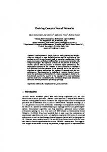
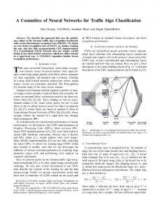
The compressed network encoding reduces the search space dimensionality by exploiting the inherent regularity in the environment. Since, as with most natural images, the pixels in a given neighborhood tend to have correlated values, searching for each weight independently is overkill. Using fewer coefficients than weights sacrifices some expressive power (some networks can no longer be represented), but constrains the search to the subspace of lower complexity, but still sufficiently powerful networks, reducing the search space dimensionality by, e.g. a factor of more than 5000 for the car-driving networks evolved here. Figure 8(a) shows the weights from the input layer of a successful car-driving network. Each 64×64 square corresponds to the input weight values of a particular neuron in the 16×16 hidden layer. The pattern in each square indicates the part of the input image to which the neuron responds. Because of the 4D structure of the input coefficient matrix, these feature detectors vary smoothly across the layer. This regularity is apparent in all five of the network matrices. Figures 8(b) and 8(c) show the activation of the hidden layer while driving through a left and right curve on the track, respectively. The two curves produce very different activation patterns from which the network computes the control signal. The highly activated neurons (in orange) form contiguous regions due to the correlation between the feature detectors of adjacent neurons. Further experiments are needed to compare the approach with other indirect or generative encodings such as HyperNEAT [2]; not only to evaluate the relative efficiency of each algorithm, but also to understand how the methods differ in the type of solutions they produce. Part of that comparison should involve testing the controllers in different conditions from those under which they were evolved (e.g. on different tracks) to measure the degree to which the ability to generalize benefits from the low-complexity representation, as was shown in [10]. In this work, the size of the networks was decided heuristically. In the future, we would like to apply Compressed
Figure 5: Visual TORCS network controller pipeline. At each time-step a raw 64×64 pixel image, taken from the driver’s perspective, is split into three planes (hue, saturation and brightness). The saturation plane is then passed through Robert’s edge detector [12] and then fed into the 16×16=256 recurrent neurons of the controller network, which then outputs the three driving commands. Network Complexity Search [5] to simultaneously determine the number of coefficients and the number of neurons (topology) by running multiple evolutionary algorithms in parallel, one for each topology-coefficient complexity class, and assigning run-time to each based on a probability distribution that is adapted on-line according to the performance of each class. This approach has so far only been applied to much simpler control tasks than those used here, but should produce solutions for harder tasks that are both simple in terms of weight matrix regularity, and model class, to evolve potentially more robust controllers. The compressed network encoding used here assumes bandlimited networks, where the matrices can contain all frequencies up to a predefined limit frequency. For networks with as many weights as those used for visual TORCS, this may not be the best scheme as the limit has to be chosen by the user, and if some specific high frequency is needed to solve the task, then all lower frequencies must be searched as well. A potentially more tractable approach might be Generalized Compressed Network Search (GCNS; [14]) which uses a messy GA to simultaneously determine which arbitrary subset of frequencies should be used as well as the value at each of those frequencies. Our initial work with this method has been promising.
Figure 7: Visual TORCS results. Typical fitness evolution of a compressed (upper curve) and directly encoded (lower curve) controller during 1000 generations. The compressed controller escapes from the local minima at generation 118, but the directly encoded network never learns to distinguish between left and right curve from the visual features.
(b)
(a)
(c)
Figure 8: Evolved low-complexity feature detectors. (a) each square shows the 64×64 input weight values corresponding to one of the neurons in 16×16 hidden layer. Colors indicate weight value: orange = large positive; blue = large negative. (b) the activation of each neuron in the hidden layer while the car is being driven through and left curve, and (c) during a right curve.
Acknowledgements This research was supported by Swiss National Science Foundation grants #137736: “Advanced Cooperative NeuroEvolution for Autonomous Control” and #138219: “Theory and Practice of Reinforcement Learning 2”. Koutn´ık implemented the compressed networks based on original ideas from our previous work cited here, and conducted the experiments. Schmidhuber supervised Koutn´ık. Cuccu devised and implemented the extensive modifications to the TORCS simulator. Gomez directed this research, and wrote most of the paper.
References [1] G. Cuccu, M. Luciw, J. Schmidhuber, and F. Gomez. Intrinsically motivated evolutionary search for visionbased reinforcement learning. In Proceedings of the IEEE Conference on Development and Learning, and Epigenetic Robotics, 2011. [2] D. B. D’Ambrosio and K. O. Stanley. A novel generative encoding for exploiting neural network sensor and output geometry. In Proceedings of the 9th annual conference on Genetic and evolutionary computation, (GECCO), pages 974–981, New York, NY, USA, 2007. ACM. [3] J. Gauci and K. Stanley. Generating large-scale neural networks through discovering geometric regularities. In Proceedings of the Conference on Genetic and Evolutionary Computation, pages 997–1004, New York, NY, USA, 2007. ACM. ISBN 978-1-59593-697-4. doi: http://doi.acm.org/10.1145/1276958.1277158. [4] F. Gomez, J. Schmidhuber, and R. Miikkulainen. Accelerated neural evolution through cooperatively coevolved synapses. Journal of Machine Learning Research, 9(May):937–965, 2008. [5] F. Gomez, J. Koutn´ık, and J. Schmidhuber. Compressed network complexity search. In Proceedings of the 12th International Conference on Parallel Problem Solving from Nature (PPSN XII, Taormina, IT), 2012. [6] F. Gruau. Cellular encoding of genetic neural networks. Technical Report RR-92-21, Ecole Normale Superieure de Lyon, Institut IMAG, Lyon, France, 1992.
[7] H. Kitano. Designing neural networks using genetic algorithms with graph generation system. Complex Systems, 4:461–476, 1990. [8] J. Koutn´ık, F. Gomez, and J. Schmidhuber. Searching for minimal neural networks in fourier space. In Proceedings of the 4th Annual Conference on Artificial General Intelligence, 2010. [9] J. Koutn´ık, F. Gomez, and J. Schmidhuber. Evolving neural networks in compressed weight space. In Proceedings of the Conference on Genetic and Evolutionary Computation (GECCO), 2010. [10] J. Koutn´ık, J. Schmidhuber, and F. Gomez. A frequency-domain encoding for neuroevolution. Technical report, arXiv:1212.6521, 2012. [11] D. Loiacono, P. L. Lanzi, J. Togelius, E. Onieva, D. A. Pelta, M. V. Butz, T. D. L¨ onneker, L. Cardamone, D. Perez, Y. S´ aez, M. Preuss, and J. Quadflieg. The 2009 simulated car racing championship, 2009. [12] L. G. Roberts. Machine Perception of ThreeDimensional Solids. Outstanding Dissertations in the Computer Sciences. Garland Publishing, New York, 1963. ISBN 0-8240-4427-4. [13] J. Schmidhuber. Discovering neural nets with low Kolmogorov complexity and high generalization capability. Neural Networks, 10(5):857–873, 1997. [14] R. K. Srivastava, J. Schmidhuber, and F. Gomez. Generalized compressed network search. In Proceedings of the 12th International Conference on Parallel Problem Solving from Nature (PPSN XII, Taormina, IT), 2012. [15] V. V. Tolat and B. Widrow. An adaptive “broom balancer” with visual inputs. In Proceedings of the IEEE International Conference on Neural Networks (San Diego, CA), pages 641–647. Piscataway, NJ: IEEE, 1988. [16] Y. Yekutieli, R. Sagiv-Zohar, R. Aharonov, Y. Engel, B. Hochner, and T. Flash. A dynamic model of the octopus arm. I. biomechanics of the octopus reaching movement. Journal of Neurophysiology, 94(2):1443– 1458, 2005.