Evolving Neural Networks for the Classification of Galaxies
Erick Cant´ u-Paz and Chandrika Kamath Center for Applied Scientific Computing Lawrence Livermore National Laboratory Livermore, CA 94551 cantupaz,
[email protected]
1
Abstract
are approximately 90 radio-emitting galaxies, or radio sources, in a typical square degree.
The FIRST survey (Faint Images of the Radio Sky at Twenty-cm) is scheduled to cover 10,000 square degrees of the northern and southern galactic caps. Until recently, astronomers classified radio-emitting galaxies through a visual inspection of FIRST images. Besides being subjective, prone to error and tedious, this manual approach is becoming infeasible: upon completion, FIRST will include almost a million galaxies. This paper describes the application of six methods of evolving neural networks (NNs) with genetic algorithms (GAs) to identify bentdouble galaxies. The objective is to demonstrate that GAs can successfully address some common problems in the application of NNs to classification problems, such as training the networks, choosing appropriate network topologies, and selecting relevant features. The results indicate that most of the methods we tried performed equally well on our data, but using a GA to select features produced the best results.
Radio sources exhibit a wide range of morphological types that provide clues to the source’s class, emission mechanism, and properties of the surrounding medium. Sources with a bent-double morphology are of particular interest as they indicate the presence of clusters of galaxies, a key project within the FIRST survey. FIRST scientists currently identify the bentdouble galaxies by visual inspection, which—besides being subjective, prone to error and tedious—is becoming increasingly infeasible as the survey grows.
INTRODUCTION
The Faint Images of the Radio Sky at Twenty-cm (FIRST) survey (Becker et al., 1995) started in 1993 with the goal of producing the radio equivalent of the Palomar Observatory Sky Survey. Using the Very Large Array at the National Radio Astronomy Observatory, FIRST is scheduled to cover more than 10,000 square degrees of the northern and southern galactic caps. At present, FIRST has covered about 8,000 square degrees, producing more than 32,000 twomillion pixel images. At a threshold of 1 mJy, there
Our goal is to bring automation to the classification of galaxies using techniques from data mining, such as neural networks. Neural networks (NNs) have been used successfully to classify objects in many astronomical applications (Odewahn et al., 1992; StorrieLombardi et al., 1992; Adams & Woolley, 1994). However, the success of NNs largely depends on their architecture, their training algorithm, and the choice of features used in training. Unfortunately, determining the architecture of a neural network is a trial-anderror process; the learning algorithms must be carefully tuned to the data; and the relevance of features to the classification problem may not be known a priori. Our objective is to demonstrate that genetic algorithms (GAs) can successfully address the topology selection, training, and feature selection problems, resulting in accurate networks with good generalization abilities. This paper describes the application of six combinations of genetic algorithms and neural networks to the identification of bent-double galaxies. This study is one of a handful that compares different methods to evolve neural nets on the same domain (Roberts & Turenga, 1995; Siddiqi & Lucas, 1998; Gr¨onross, 1998). In contrast with other studies that limit their scope to two or three methods, we compare six combinations of GAs and NNs against hand-
designed networks. Most of the methods we tried performed equally well on our data, but using a GA to select features yielded the best results. The experiments also show that most of the GA and NN combinations produced significantly more accurate classifiers than we could obtain by designing the networks by hand. The next section outlines the problem of detecting bent-double galaxies in the FIRST data. Section 3 describes several existing combinations of GAs and NNs. Section 4 presents our experiments and reports the results. The paper concludes with our observations and plans for future work.
2
FIRST SURVEY DATA
Figure 1 has several examples of radio sources from the FIRST survey. While some bent-double galaxies are relatively simple in shape (examples (a) and (b)), others, such as the ones in examples (e) and (f), can be rather complex. Note the similarity between the bent-double in example (a) and the non-bent-double in example (c). Data from FIRST are available on the FIRST web site (sundog.stsci.edu). There are two forms of data available: image maps and a catalog. The images in figure 1 are close-ups of galaxies. The catalog (White et al., 1997) is obtained by fitting two-dimensional Gaussians to each radio source on an image map. Each entry in the catalog corresponds to a single Gaussian. We decided that, initially, we would identify the radio sources and extract the features using only the catalog. The astronomers expected that the catalog was a good approximation to all but the most complex of radio sources, and several of the features they thought were important in identifying bent-doubles were easily calculated from the catalog. We identified the features for the bent-double problem through extensive conversations with FIRST astronomers. When they justified their decisions of identifying a radio source as a bent-double, they placed great importance on spatial features such as distances and angles. Frequently, the astronomers would characterize a bent-double as a radio-emitting “core” with one or more additional components at various angles. In the past, we have concentrated our work on instances described by three catalog entries, because we have more labeled examples of this type. Our previous experience with this data suggested that the best accuracies are usually achieved using features extracted considering triplets of catalog entries (as opposed to pairs or single entries). Therefore, in the remainder
of this paper we focus on the 20 triplet features that we extracted. A full list of features is described elsewhere (Fodor et al., 2000). Unfortunately, our training set is relatively small, containing 195 examples for the three-catalog entry sources. Since the bent- and non-bent-doubles must be manually labeled by FIRST scientists, putting together an adequate training set is non-trivial. Moreover, scientists are usually subjective in their labeling of galaxies, and the astronomers often disagree in the hard-to-classify cases. There is also no ground truth we can use to verify our results. These issues imply that the training set itself is not very accurate, and there is a limit to the accuracy we can obtain. Among the 195 labeled examples of 3-entry sources, 28 are non-bent and 167 are bent-double galaxies. This unbalanced distribution in the training set presents problems in estimating the accuracy of the NNs, which are discussed in section 4.
3
GENETIC NEURAL NETWORKS
Genetic algorithms and neural networks have been used together in several ways, and this section presents a brief review of previous work. In particular, GAs have been used to search for the weights of the network and to select the most relevant features of the training data. GAs have also been used to design the structure of the network. It is well known that to solve nonlinearly separable problems, the network must have at least one hidden layer between the inputs and outputs; but determining the number and the size of the hidden layers is mostly a matter of trial and error. GAs have been used to search for these parameters, as well as for the pattern of connections and for developmental instructions to generate a network. The interested reader may consult the reviews by Branke (1995), Schaffer (1994) and Yao (1999). 3.1
TRAINING NETWORKS WITH GAs
Training a NN is an optimization task with the goal of finding a set of weights that minimizes an error measure. The search space is high dimensional and, depending on the error measure, it may contain numerous local optima. Some network training algorithms, such as backpropagation (BP), use some form of gradient search, and may get trapped in local optima. A straightforward combination of genetic algorithms and neural networks is to use the GA to search for weights that make the network perform as desired. The architecture of the network is fixed by the user
(a)
(b)
(c)
(d)
(e)
(f)
Figure 1: Example radio sources: (a)-(b) Bent-doubles, (c)-(d) Non-bent doubles, (e)-(f) Complex Sources prior to the experiment. In this method, each individual in the GA represents a vector with all the weights of the network. There are two popular variations: • Use the weights found by the GA without any further refinement (Caudell & Dolan, 1989; Montana & Davis, 1988; Whitley & Hanson, 1989). • Use the GA to find a promising set of weights from which a gradient-based method can quickly reach an optimum (Skinner & Broughton, 1995). The motivation is that GAs quickly identify promising regions of the search space, but they may not finetune parameters very fast. These approaches are straightforward and numerous studies report good results. However, since adjacent layers in a network are usually fully connected, the total number of weights is O(n2 ), where n is the number of units. Longer individuals usually require larger populations, which in turn result in higher computational costs. Therefore, the GA may be efficient for small networks, but this method may not scale up well. Another drawback is the so-called permutations problem (Radcliffe, 1990). The problem is that by permuting the hidden nodes of a network, the representation of the weights in the chromosome would change, but the network is functionally the same. Some permutations may not be suitable for GAs because crossover might easily disrupt favorable combinations of weights. To ameliorate this problem, Thierens et al. (1991) suggested to
place incoming and outgoing weights of a hidden node next to each other, which was the encoding we used. 3.2
FEATURE SELECTION
Besides searching for weights, GAs may be used to select the features that are input to the NNs. The training examples may contain irrelevant or redundant features, but it is generally unknown a priori which features are relevant. Avoiding irrelevant or redundant features is desirable not only because they increase the size of the network and the training time, but also because they may reduce the accuracy of the network. Applying GAs to select features is straightforward using what is referred to as the wrapper approach: the chromosome of the individuals contains one bit for each feature, and the value of the bit determines whether the feature will be used in the classification (Brill, Brown, & Martin, 1990; Brotherton & Simpson, 1995). The individuals are evaluated by training the networks (that have a predetermined structure) with the subset of features indicated by the chromosome. The resulting accuracy estimate is used to calculate the fitness. 3.3
DESIGNING NETWORKS WITH GAs
As mentioned before, the topology of a network is crucial to its performance. If a network has too few nodes and connections, it may not be able to learn the re-
quired concept. On the other hand, if a network has too many nodes and connections, it may overfit the training data and have poor generalization. GAs have been used successfully to design the topology of NNs. There are two basic approaches for applying GAs to the design of NNs: use a direct encoding to specify every connection of the network or evolve an indirect specification of the connectivity. The key idea behind direct encodings is that a neural network can be regarded as a directed graph where each node represents a neuron and each edge is a connection. A common method of representing directed graphs is with a binary connectivity matrix: the i, jth element of the matrix is one if there is an edge between nodes i and j, and zero otherwise. The connectivity matrix can be represented in a GA simply by concatenating its rows or columns (Miller et al., 1989; Belew et al., 1990). Using this method, Whitley et al. (1990) showed that the GA can find topologies that learn faster than the typical fully-connected feedforward network. The GA can be explicitly biased to favor smaller networks, which can be trained faster. A simple method to avoid specifying all the connections is to commit to a particular topology and learning algorithm, and then use the GA to find the parameter values that complete the network specification. For example, with a fully-connected feedforward topology, the GA may search for the number of layers and the number of neurons per layer. Another example would be to code the parameters of a particular learning algorithm, such as the momentum and the learning rate of BP (Belew et al., 1990; Marshall & Harrison, 1991). Of course, this method is constrained by the initial choice of topology and learning algorithm. Another approach is to use a grammar to encode rules that govern the development of a network. Kitano (1990) introduced the earliest grammar-based approach. He used a connectivity matrix to represent the network, but instead of encoding the matrix directly in the chromosome, the matrix is generated by a graphrewriting grammar. The chromosomes contain rules that rewrite scalar elements into 2 × 2 matrices. In this grammar, there are 16 terminal symbols that are 2 × 2 binary matrices. There are 16 non-terminal symbols, and the rules have the form n → m, where n is one of the scalar non-terminals, and m is a 2 × 2 matrix of non-terminals. There is an arbitrarily designated start symbol, and the number of rewriting steps is fixed by the user. To evaluate the fitness, the rules are decoded and the connectivity matrix is developed by applying all the
rules that match non-terminal symbols. Then, the connectivity matrix is interpreted and the network is constructed and trained with BP. Other examples of grammar-based developmental systems are the work of Boers and Kuiper (1992) with Lindenmayer systems, Gruau’s “cellular encoding” method (Gruau, 1992), and the system of Nolfi, Elman, and Parisi (1994) that simulates cell growth, migration, and differentiation.
4
EXPERIMENTS
This section details the experimental methods and the results that we obtained with six combinations of neural networks and genetic algorithms. The programs were written in C++ and compiled with g++ version 2.96. The experiments were executed on a single processor of a Linux (Red Hat 7.1) workstation with dual 1.5 GHz Intel Xeon processors and 512 Mb of memory. The programs used a Mersenne Twister random number generator. All the GAs used a population of 50 individuals. We used a simple GA with binary encoding, pairwise tournament selection, and multi-point crossover. The number of crossover points was varied in each experiment according to the length of the chromosomes, l. In all cases, the probability of crossover was 1, and the probability of mutation was set to 1/l. The initial population was initialized uniformly at random. The experiments used feedforward networks with one hidden layer. All neurons are connected to a “bias” unit with constant output of 1.0. Unless specified otherwise, the output units are connected to all the hidden units, which in turn are connected to all the inputs. In feedforward operation, the units compute their net activation as d X net = x i wi + w 0 , i=1
where d is the number of inputs to the neuron, xi is an input and wi is the corresponding weight, w0 is the weight corresponding to the “bias” unit. Each unit emits an output according to f (net) = tanh(β ∗ net), where β is a user-specified coefficient. Simple backpropagation was used in some of the experiments. The weights from the hidden to the output layer were updated using ∆wkj = ηδk yj = η(tk − zk )f 0 (netk )yj , where η denotes the learning rate, k indexes the output units, tk the desired output, zk the actual output, f 0 is the derivative of f , and yj is the output of the j-th hidden unit. The weights from the i-th input to the
hidden layer were updated using # " c X ∆wji = η wkj δk f 0 (netj )xi . k=1
In all experiments, each feature in the data was linearly normalized to the interval [−1, 1]. The type of galaxy was encoded in one output value (-1 for bent and 1 for non-bent). When backpropagation was used, the examples were presented in random order for 20 epochs. All the results reported are averages over 10 runs of the algorithms. Comparisons were made using standard t-tests with 95% confidence. 4.1
FITNESS CALCULATION
One of the crucial design decisions for the application of GAs is the calculation of fitness values for each member of the population. Since we are interested in networks that predict accurately the type of galaxies not used in training, the fitness calculation must include an estimate of the generalization ability of the networks. There are multiple ways to estimate generalization. Since we do not have much training data, hold-out methods (dividing the data into training and testing sets and perhaps an additional validation set) are not practical. To calculate the fitness, we used the accuracy estimate of five-fold crossvalidation trials. In this method, the data D is divided into five nonoverlapping sets, D1 , ..., D5 . At each iteration i (from 1 to 5), the network is trained with D\Di and tested on Di . The average of the five tests was used as the fitness. A better estimate of accuracy would be to use an average of multiple crossvalidation experiments, but we found the cost excessive. To correct for the unbalanced distribution of bent and non-bent examples in our training data, we calculate the accuracy as the geometric mean of the accuracies of each class of galaxy (bent and non-bent) (Kubat & Matwin, 1997). Using the geometric mean gives equal weight to the accuracies on both types of galaxies in the overall performance. 4.2
TRAINING NETWORKS WITH GAs
We implemented the first of the methods described in section 3.1: the GA was used to find the network’s weights. The network had 20 inputs that correspond to each of the features in the data, 25 hidden nodes, and one output. Each weight was represented with 10 bits, and the range of possible weights was [−10, 10]. For this experiment, the GA used a population of 50 individuals, each with a length of l = 5510 bits (there
are 551 total weights). The number of crossover points was set at 25, and the mutation rate was 0.00018 (≈ 1/l). As in all experiments, pairwise tournament selection without replacement was used. The second training method described in section 3.1 is to run BP using the weights represented by the individuals in the GA to initialize the network. We implemented this method and used the same network architecture and GA parameters as in the first experiment. Each network was trained using 20 epochs of BP with a learning rate η of 0.1 and β of 0.4. The entries Weights and Weights+BP in table 1 present the average accuracy of the best networks found in each run of the GA for these two sets of experiments. The results highlighted in bold in the table are the best results and those not significantly worse than the best (according to the t-test, which may detect more differences than there actually exist). The addition of BP produces a significant improvement in the bent-double accuracy rate, which is of primary importance to the astronomers. However, the improvement in the overall accuracy is not significant. 4.3
FEATURE SELECTION
The next combination of GAs and NNs is to use the GA to select the features that will be used to train the networks, as described in section 3.2. As in the previous experiment, we set the number of hidden units to 25, the learning rate η to 0.1 and β to 0.4. The networks were trained with 20 epochs of BP. Our data has 20 features, and therefore the chromosomes in the GA are 20 bits long. The GA used onepoint crossover and the same parameters as in previous experiments. The accuracy results are labeled Feature Sel and are significantly better than the other results in table 1. The GAs consistently selected about half of the features, and frequently selected features that appear to be relevant to the identification of bent-double galaxies, such as symmetry measures and angles. 4.4
DESIGNING NETWORKS WITH GAs
For our first application of GAs to network design, the GA was used to find the number of hidden units, the parameters for BP, and the range of initial weights as described in section 3.3. The learning rate was encoded with four bits and the range of possible values was [0, 1]. The coefficient β for the activation function was also encoded with four bits and its range was [0, 1]. The upper and lower ranges for the initial weights were
encoded with five bits each and were allowed to vary in [−10, 0] and [0, 10], respectively. Finally, the number of hidden units was represented with seven bits and could take values in [0, 127].
pear to be significantly less accurate. In terms of the accuracy on the non-bents and the overall accuracy, it is clear that the feature selection method obtained the best results.
After extracting the parameters from a chromosome, a network was built and initialized according to the parameters and trained with 20 epochs of BP. There is no explicit bias to prefer smaller networks, but there is an implicit bias toward networks that can learn quickly, since we are using only 20 epochs of BP. It is probable that small networks learn faster than larger ones, and so it is likely that the GA favors small networks.
We also performed numerous experiments with networks designed by hand. The best parameters that we could find for 20 epochs of backpropagation were those used in the experiments with the GAs: β = 0.1, the learning rate was 0.4, and the number of hidden was 25. The average of ten 10-fold crossvalidation experiments resulted in an accuracy on the non-bents of only 16.4% (with std. error of 1.7) and on the bents of 99.69% (0.16). The overall accuracy estimated with the geometric mean is a disappointing 23.41% (2.02).
The GA used two-point crossover and the same parameters as in previous experiments. The accuracy results are labeled Parameters in table 1. On average, the best learning rate found by the GA was 0.82 (with 0.06 std. error), which is higher than the usual recommendation of 0.1–0.2 (Duda, Hart, & Stork, 2001). Perhaps the learning rate is high because of the implicit bias for learning quickly. This bias may also explain the average number of hidden units being relatively small at 15.6 (std. error 2.8). The average β was 0.16 (0.01), and the range of initial weights was [−3.51, 3.45] (both with std. errors of 0.4). The next experiment used the GA to search for a connectivity matrix as described in section 3.3. We fixed the number of hidden units to 25, the learning rate to 0.1 and β to 0.4. The neurons are numbered consecutively starting with the inputs and followed by the hidden units and outputs. The connectivity matrix is encoded by concatenating its rows. Since we allow direct connections between the inputs and the outputs, the string length is (hidden + outputs) ∗ inputs + hidden ∗ outputs = (26∗20)+(25∗1) = 545 bits. For this longer string, we use 10 crossover points, and the same GA parameters as before. The results corresponding to this method are labeled Matrix in table 1. We also implemented Kitano’s graph rewriting grammar method. We limited the number of rewriting steps to 6, resulting in networks with at most 64 units. Since the chromosomes encode four 2 × 2 binary matrices for each of the 16 rules, the string length is 256 bits. The GAs used five crossover points. The results obtained with this method are labeled Grammar in table 1. 4.5
COMPARISON AND DISCUSSION
Table 1 summarizes the results obtained with each method. The results show few differences among the various methods in the accuracy rate for bent-doubles. While the direct encoding of connections (Matrix) has the best accuracy, four other methods do not ap-
Increasing the number of training epochs to 100 raised the standard the geometric mean accuracy to 72.69% (0.32). The accuracy on the non-bents also improved to 56.7%, while the accuracy on the bents decreased slightly to 94.38%.
5
CONCLUSIONS
This paper presented a comparison of six combinations of GAs and NNs for the identification of bent-double galaxies in the FIRST survey. Our experiments suggest that, for this application, some combinations of GAs and NNs can produce accurate classifiers that are competitive with networks designed by hand. For our application, we found few differences among the GA and NN combinations that we tried. The only consistently best method was to use the GA to select the features used to train the networks, which suggests that some of the features in the training set are irrelevant or redundant. There are several avenues to extend this work. The highly unbalanced training set presents some difficulties that could be avoided or ameliorated by including more examples of the minority class. However, extending the training set is non-trivial, because the labeling is subjective and disagreements among the experts are common. Other optimization techniques, evolutionary and traditional, can be used to train NNs. In this paper we used a simple genetic algorithm with a binary encoding, but other evolutionary algorithms operate on vectors of real numbers that can be directly mapped to the network’s weights or the BP parameters (but not to a connectivity matrix, a grammar, or a feature selection application). There are other combinations of GAs and NNs that we did not include in this study, but appear promising. For instance, since evolutionary algorithms use a population of networks, a natural
Method Weights Weights+BP Feature Sel Parameters Matrix Grammar
Bent-Doubles 86.34 (2.83) 91.89 (0.67) 92.99 (0.55) 92.35 (0.89) 93.58 (0.46) 92.84 (0.69)
Non-Bent 78.01 (4.13) 75.23 (0.87) 83.65 (1.41) 69.13 (1.56) 70.77 (1.34) 73.73 (1.40)
Overall 80.98 (2.41) 81.68 (0.53) 87.51 (0.77) 78.76 (0.57) 80.22 (0.69) 81.78 (0.72)
Table 1: Mean accuracies on the bent and non-bent doubles and overall accuracy for different combinations of GAs and NNs using the geometric mean of class-wise accuracies as fitness. The numbers in parenthesis are the standard errors, and the results in bold are the best and those not significantly worse than the best. extension of this work would be to use evolutionary algorithms to create ensembles that combine several NNs to improve the accuracy of classifications. A disadvantage of using genetic algorithms in combination with neural networks is the long computation time required. This can be an obstacle to applying these techniques to larger data sets, but there are numerous alternatives to improve the performance of genetic algorithms. For instance, we could approximate the fitness evaluation using sampling or we can exploit the inherently parallel nature of GAs using multiple processors.
Acknowledgments We gratefully acknowledge our FIRST collaborators Robert Becker, Michael Gregg, David Helfand, Sally Laurent-Muehleisen, and Richard White for their technical interest and support of this work. We would also like to thank Imola K. Fodor and Nu Ai Tang for useful discussions and computational help. UCRL-JC-147020. This work was performed under the auspices of the U.S. Department of Energy by University of California Lawrence Livermore National Laboratory under contract No. W-7405-Eng-48.
References Adams, A., & Woolley, A. (1994). Hubble classification of galaxies using neural networks. Vistas in Astronomy, 38 , 273–280. Becker, R. H., White, R., & Helfand, D. (1995). The FIRST survey: Faint images of the radio sky at twenty-cm. Astrophysical Journal , 450 , 559. Belew, R., McInerney, J., & Schraudolph, N. (1990). Evolving networks: Using the genetic algorithm with connectionist learning (Tech. Rep. No. CS90174). San Diego: University of California, Computer Science and Engineering Department.
Boers, J. W., & Kuiper, H. (1992). Biological metaphors and the design of modular artificial neural networks. umt, Leiden University, The Netherlands. Branke, J. (1995). Evolutionary algorithms for neural network design and training (Technical Report). Karlsruhe, Germany: Institute AIFB, University of Karlsruhe. Brill, F. Z., Brown, D. E., & Martin, W. N. (1990). Genetic algorithms for feature selection for counterpropogation networks (Tech. Rep. No. IPC-TR90-004). Charlottesville: University of Virginia, Institute of Parallel Computation. Brotherton, T. W., & Simpson, P. K. (1995). Dynamic feature set training of neural nets for classification. In McDonnell, J. R., Reynolds, R. G., & Fogel, D. B. (Eds.), Evolutionary Programming IV (pp. 83–94). Cambridge, MA: MIT Press. Caudell, T. P., & Dolan, C. P. (1989). Parametric connectivity: Training of constrained networks using genetic algorithms. In Schaffer, J. D. (Ed.), Proceedings of the Third International Conference on Genetic Algorithms (pp. 370–374). San Mateo, CA: Morgan Kaufmann. Duda, R. O., Hart, P. E., & Stork, D. G. (2001). Pattern classification. New York, NY: John Wiley & Sons. Fodor, I. K., Cant´ u-Paz, E., Kamath, C., & Tang, N. (2000). Finding bent-double radio galaxies: A case study in data mining. In Interface: Computer Science and Statistics, Volume 33. Gr¨onross, M. A. (1998). Evolutionary design of neural networks. Unpublished master’s thesis, University of Turku. Gruau, F. (1992). Genetic synthesis of boolean neural networks with a cell rewritting developmental process. In Whitley, D., & Schaffer, J. D. (Eds.), Proceedings of the International Workshop on Com-
binations of Genetic Algorithms and Neural Networks (pp. 55–74). Los Alamitos, CA: IEEE Computer Society Press.
Iternational Conference on Evolutionary Computation (pp. 392–397). Piscataway, NJ: IEEE Service Center.
Kitano, H. (1990). Designing neural networks using genetic algorithms with graph generation system. Complex Systems, 4 (4), 461–476.
Skinner, A., & Broughton, J. Q. (1995). Neural networks in computational material science: training algorithms. Modelling and Simulation in Material Science and Enginnering, 3 , 371–390.
Kubat, M., & Matwin, S. (1997). Addressing the curse of imbalanced training sets: One-sided selection. In Proceedings of the 14th International Conference on Machine Learning (pp. 179–186). San Francisco, CA: Morgan Kaufmann. Marshall, S. J., & Harrison, R. F. (1991). Optimization and training of feedforward neural networks by genetic algorithms. In Proceedings on the Second International Conference on Artifical Neural Networks and Genetic Algorithms (pp. 39–43). Springer Verlag. Miller, G. F., Todd, P. M., & Hegde, S. U. (1989). Designing neural networks using genetic algorithms. In Schaffer, J. D. (Ed.), Proceedings of the Third International Conference on Genetic Algorithms (pp. 379–384). San Mateo, CA: Morgan Kaufmann. Montana, D. J., & Davis, L. (1988). Training feedforward neural networks using genetic algorithms. unpublished manuscript. Nolfi, S., Elman, J. L., & Parisi, D. (1994). Learning and evolution in neural networks (Tech. Rep. No. 94-08). Rome, Italy: Institute of Psychology, National Research Council. Odewahn, S., Stockwell, E., Pennington, R., Humphreys, R., & Zumach, W. (1992). Automated star/galaxy discrimination with neural networks. The Astronomical Journal , 103 (1), 318–331. Radcliffe, N. J. (1990). Genetic neural networks on MIMD computers. Unpublished doctoral dissertation, University of Edinburgh, Scotland. Roberts, S. G., & Turenga, M. (1995). Evolving neural network structures. In Pearson, D., Steele, N., & Albrecht, R. (Eds.), International Conference on Genetic Algorithms and Neural Networks (pp. 96– 99). New York: Springer-Verlag. Schaffer, J. D. (1994). Combinations of genetic algorithms with neural networks or fuzzy systems. In Zurada, J. M., Marks, II, R. J., & Robinson, C. J. (Eds.), Computational Intelligence Imitating Life (pp. 371–382). New York, NY: IEEE Press. Siddiqi, A. A., & Lucas, S. M. (1998). A comparison of matrix rewriting versus direct encoding for evolving neural networks. In Proceedings of 1998 IEEE
Storrie-Lombardi, M., Lahav, O., Sodre, L., & StorrieLombardi, L. (1992). Morphological classification of galaxies by artificial neural networks. Mon. Not. R. Astron. Soc., 259 , 8–12. Thierens, D., Suykens, J., Vandewalle, J., & Moor, B. D. (1991). Genetic weight optimization of a feedforward neural network controller. In Proceedings of the Conference on Neural Nets and Genetic Algorithms (pp. 658–663). Springer Verlag. White, R. L., Becker, R., Helfand, D., & Gregg, M. (1997). A catalog of 1.4 GHz radio sources from the FIRST survey. Astrophysical Journal , 475 , 479. Whitley, D., & Hanson, T. (1989). Optimizing neural networks using faster, more accurate genetic search. In Schaffer, J. D. (Ed.), Proceedings of the Third International Conference on Genetic Algorithms (pp. 391–397). San Mateo, CA: Morgan Kaufmann. Whitley, D., Starkweather, T., & Bogart, C. (1990). Genetic algorithms and neural networks: Optimizing connections and connectivity. Parallel Computing, 14 , 347–361. Yao, X. (1999). Evolving artificial neural networks. Proceedings of the IEEE , 87 (9), 1423–1447.