Brighton Innovation Centre. University of Sussex, Falmer, Brighton, BN1 9QG, U.K.. Abstract .... giving the robots a top speed of around 6cm/s. An un- powered castor .... The final component of a team's trial score, the scalar st, is a measure of ...
Evolving Team Behaviour for Real Robots. Matt Quinn∗ ∗
Lincoln Smith∗
Phil Husbands∗
† Mathematique Appliqu´e S.A. Centre for Computational Neuroscience and Robotics, Brighton Innovation Centre. and School of Cognitive and Computing Sciences. University of Sussex, Falmer, Brighton, BN1 9QG, U.K.
Abstract We report on recent work in which we employed artificial evolution to design neural network controllers for small, homogeneous teams of mobile autonomous robots. The robots are evolved to perform a formation movement task from random starting positions, equipped only with infrared sensors. The dual constraints of homogeneity and minimal sensors make this a non-trivial task. We describe the behaviour of a successful evolved team in which robots adopt and maintain functionally distinct roles in order to achieve the task. We believe this to be the first example of the use of artificial evolution to design coordinated, cooperative behaviour for real robots.
1
Giles Mayley†
Introduction
In this paper we report on our recent work evolving controllers for robots which are required to work as a team. The word ‘team’ has been used in a variety of senses in both the multi-robot and the ethology literature, so it is appropriate to start the paper with a definition. We will adopt the definition given by Anderson and Franks in their recent review of team behaviour in animal societies. They identify three of defining features of team behaviour. Firstly, individuals make different contributions to task success, i.e. they perform different subtasks or roles (although more than one individual may adopt the same role). Secondly, individual roles or sub-tasks are interdependent (or “interlocking”) requiring structured cooperation; individuals operate concurrently, coordinating their different contributions in order to complete the task. Finally, a team’s organisational structure persists over time, although its individuals may be substituted, or swap roles (Anderson and Franks, 2001). The designer of a multi-robot team faces a number of challenges. One of which arises because a team is a structured system, robot controllers must be designed in such a way that the robots will both become and remain appropriately organised. One solution is to design a heterogeneous team, in which each individual’s role is
predetermined (e.g. Balch and Arkin, 1998). This has the additional advantage of specialisation, in that each robot’s behavioural and morphological design can be tailored to its particular task. However, we are interested in homogeneous systems, in which all robots are built to the same design, and have identical controllers. Our interest in homogeneous teams stems from their potential for system-level robustness and graceful degradation which results from their complete lack of specialisation— although we do not address this issue in this paper. The constraint of homogeneity makes the design task more difficult, since there are no differences between robots’ control systems or morphologies which can be exploited for the purposes of team organisation. Other mechanisms must thus be employed to facilitate the dynamic allocation, maintenance and coordination of roles. Dynamic role allocation and structured co-operation are areas which have been addressed by a number of researchers in the field of multi-robot systems, involving successful implementations of such tasks as cooperative transport (Chaimowicz et al., 2001), robot football (Stone and Veloso, 1999) and coordinated movement (Matari´c, 1995). In such cases, design solutions have relied heavily on the use of global information shared by radio communication. For example, in Matari´c’s implementation of coordinated movement with homogeneous robots, robots made use of a common coordinate system (through radio beacon triangulation) and exchanged positional information via radio communication in order to remain coordinated (Matari´c, 1995). In the case of dynamic role or task allocation, solutions have relied on radio communication protocols to coordinate role allocation, with the appropriate coordination and allocation of roles relying on robots globally advertising or negotiating their current (or intended) roles (see e.g. Chaimowicz et al., 2001; Stone and Veloso, 1999). Our work differs from that of these researchers. We wish to design teams in which system-level organisation arises, and is maintained, solely through local interactions between individuals which are constrained to utilise minimal and ambiguous local information. Systems capable of functioning under such constraints have some in-
teresting potential engineering applications (see, for example, Hobbs et al. (1996) for discussion of the need for minimal systems in the space industry). However, they are also interesting from an adaptive behaviour perspective, providing an example of a phenomenon often referred to as ‘self-organising’ or ‘emergent’ behaviour (Camazine et al., 2001). Imposing the joint constraints of homogeneity and minimal sensors leaves us with a complex design task. One which cannot easily decomposed and addressed by conventional ‘divide and conquer’ design methodologies. Instead, it is a problem exhibiting significant interdependence of its constituent parts. For this reason, we have adopted an evolutionary robotics approach, employing artificial evolution to automate the design process, since such an approach is not constrained by the need for decomposition or modular design. It is worth noting that—insofar as we are aware—the work reported in this paper represents the first successful use of evolutionary robotics methodology to develop cooperative, coordinated behaviour for a real multi-robot system. (See Nolfi and Floreano (2000) for a recent survey of evolutionary robotics research). The work which we will describe in this paper represents our first experiments in the evolutionary design of homogeneous multi-robot teams. We used three robots, each minimally equipped with four active infra-red sensors, and two motor-driven wheels. Robot controllers were evolved to perform a formation movement task, in an obstacle-free environment, starting from random initial positions. The robots and their task are introduced in more detail in sections 2 and 3. Robots were controlled by neural networks which were evolved in simulation, before being successfully transferred onto real robots. The networks, simulation and evolutionary machinery are covered in section 4. Section 5 describes the successful behaviour of one of the evolved teams in some detail, showing that task success is dependent on the robots performing as team, in accordance with definition given at the beginning of this paper.
2
The Robots
For these experiments, we used three robots which had been built to the same specification. Each robot is 16.75 cm square and 11 cm high. Two motor-driven wheels, made of foam-rubber, are located on either side of the robot, providing locomotion through differential drive, giving the robots a top speed of around 6cm/s. An unpowered castor wheel, placed rear-centre, ensures stability. In the experiments described in this paper, a robot’s only source of sensory input comes from its four active infrared sensors, two located at the front of the robot, and two at the rear, as shown in figure 1. The robots are controlled by a host computer, with each robot sending its sensor readings to and receiving its effector activations from this machine via a radio link.
Figure 1: Plan view of a robot, showing location of sensors and motors. Note that the CCD camera was not used in the experiments.
Each robot uses a 80C537-based micro-controller board for low-level control. The host computer is responsible for running the controller for each robot, updating each controller’s inputs with the sensor readings from the appropriate robot, and transmitting the controller’s output to the robot. In these experiments, each robot was updated at approximately 5 Hz. It should be noted that although the physical instantiation of the robots has been implemented as a host/slave system, conceptually the robots are to be considered as independent, autonomous agents by virtue of the logical division of control into distinct and self-contained controllers on the host machine.
2.1 Infrared Sensors The reader may not be familiar with the limitations of active infrared sensors, especially those peculiar to a multi-robot scenario, so we will address them in some detail. An active infrared sensor comprises a paired infrared emitter and receiver. Its normal function is to emit an infrared beam and then measure the amount of infrared which reflects back from nearby objects. In this way our robots can use their sensors to detect other robots up to a maximum of about 18cm (i.e. just over one body length away). The dark grey beams in the lefthand panel of figure 2 indicate the limited areas in which a robot can detect other robots in this manner. IR sensors are often referred to as proximity sensors, but this is somewhat misleading. Whilst the sensor reading due to reflected IR is a non-linear, function of the distance to the object detected, it is also a function of the angle at which the emitted beam strikes the surface of the object, and of the proportion of the beam which strikes that object. It is because an IR sensor reading combines these three factors into a single value that, even in normal function, sensor readings are ambiguous. The ambiguity of IR sensors is significantly increased in a multi-robot scenario, since a robot’s IR emissions can be directly sensed by other robots. The light grey beams in the left-hand panel of figure 2 indicates the approximate area in which a robot’s infrared emissions may be directly detected by other robots. The maximum range at which emissions can be detected is approximately 30cm—almost twice the range at which a robot can detect an object by reflected IR. The righthand panel of the same diagram illustrates the range of angles at which a robot can receive the IR emissions of
other robots. The sensor value due to receiving another’s IR emissions is also the combined function of a number of factors: It will depend on the distance between the robots, but also the angle at which the emitted beam strikes the other robot’s receiver, and which portion of the beam strikes the receiver (IR is significantly more intense at the centre of the beam than at the edges). Readings due to direct IR are thus ambiguous for the same reasons as reflected IR. However, ambiguity is compounded by the fact that, to the robot, readings due to reflected IR are indistinguishable from those due to the reception of IR emissions of other robots. Moreover, a sensor reading may be the result of a combination of both reflected and direct IR, and it may be due to one or both of the other robots.
direct information about a robot’s surroundings. Any given set of sensor input can be the result of any one of large number of significantly different circumstances. Furthermore, outside the limited range of their IR sensors, robots have no indication of each other’s position. Any robot straying more than two body-lengths from its teammates will cease to have any indication of their location. It should be clear that the team’s situation contrasts strongly with previous work in which robots utilised shared coordinate systems and global communication. It is worth noting that biological models of selforganising coordinated movement assume typically that agents are presented with significantly more information about their local environment than these robots have. For example, in models of flocking and shoaling, agents are typically assumed to have ideal sensors which provide the location, velocity and orientation of their nearest neighbours (reviewed in Camazine et al., 2001). The team are also constrained by their homogeneity for the reasons discussed in the introduction. The team must move from their initial random configuration into the formation which they will maintain whilst moving. In so doing it seems inevitable that different robots will be required to adopt different roles (for example, a leader and two followers). The robots must find some way of appropriately allocating and maintaining these roles despite the lack of any intrinsic differences between them. This is, of course, made all the more challenging by the poverty of the robots’ sensory input.
3
4
Figure 2: Left: The extent to which reflected IR can be sensed (dark grey area), and to which IR beam is perceptible to other robots (light grey area). Right: The angles from which a robot can perceive the IR emissions of others
The Task
The task with which we present the robots is an extension of that used in previous work which involved two simulated Khepera robots (Quinn, 2001). Adapted for three robots, the task is as follows: Initially, the three robots are placed in an obstacle-free environment in some random configuration, such that each robot is within sensor range of the others. Thereafter, the robots are required to move, as a group, a certain distance away from their initial position. During evolution robots are evaluated on their ability to move the group centroid one metre within the space of three simulated minutes. However, our expectation was that a team capable of this would be able to sustain formation movement of much longer periods. The robots are not required to adopt any particular formation, only to remain within sensor range of one another, and to avoid collisions. Since the robots start from initial random configurations, we anticipate that successful completion of the task will entail two phases. The first entailing the team organising itself into a formation, and the second entailing the team moving whilst maintaining that formation. From the characterisation of the robots’ sensors in the previous section, it should be clear that these impose significant constraints. They provide very little
Implementation
4.1 Evaluating Team Performance A single genotype was used to generate a team by ‘cloning’ (i.e. decoding the genotype and then making copies of the resulting controller). Given that different starting positions will present different challenges, it was important that each team (i.e. each evolutionary individual) is evaluated under the same set of initial conditions. To this end, at each generation of the evolutionary algorithm, a set of 100 starting positions was randomly generated, (see figure 3), and used for the evaluation of all the teams. Fitness was the average score after one trial from each starting position in the evaluation set. Figure 3: An example starting position: Each robot’s orientation is set randomly in the range [0:2π], and the minimum distance between the edges of each robot and its nearest neighbour is set randomly in the range [10:22cm].
Reflecting the task description, the evaluation function seeks to assess the ability of the team to increase
its distance from its starting position, whilst avoiding collisions and staying within sensor range. It therefore consists of three main components. First, at each timestep of the trial, the team is rewarded for any gains in distance. Second, this reward is multiplied by a dispersal scalar, reducing the fitness increment when one or more robots are outside of IR sensor range. Third, at the end of a trial, the accumulated score is reduced in proportion to the number of collisions which have occurred during that trial. More specifically, a team’s trial score, is: T h ³X ¡ ¢ ¡ ¢i ´ f dt , Dt−1 . 1 + tanh (st /20) P. t=1
Here P is a collision-penalty scalar in the range [0.5 : 1], such that, if c is the number of collisions between robots, and cmax = 20 is the maximum number of collisions allowed, then P = 1 − c/2cmax . The distance gain component is given by the function f . This measures any gain that the team have made on their previous best distance from their initial location. Here a team’s location is taken to be the centre-point (or centroid) of the group. If dt is the Euclidean distance between the group’s location at time t and its location at time t = 0, Dt−1 is the largest value that dt has attained prior to time t, and Dmax is the required distance (i.e. 100 c.m.), then the function f is defined as: ½ dt − Dt−1 if Dt−1 < dt < Dmax f (dt , Dt−1 ) = 0 otherwise The final component of a team’s trial score, the scalar st , is a measure of the team’s dispersal beyond sensor range at time t. If each robot is within sensor range of at least one other, then st = 0. Otherwise, the two shortest lines that can connect all three robots are found, and st is the distance by which the longest of these exceeds sensor range. In other words, the team is penalised for its most wayward member.
4.2 Simulation Controllers were initially evolved in simulation, before being transferred to the real robots. A big problem with evolving in simulation is that controllers may become adapted to inaccurate features of the simulation, not present in the real world. However, building a completely accurate model of the robots and their sensors and motors would be an onerous and potentially unachievable task. To avoid this problem we employed Jakobi’s minimal simulation methodology (Jakobi, 1998). This entailed building a relatively crude model of the robot and its interactions with its environment. The parameters of this model were systematically varied, within certain ranges, between each evaluation of a team. Parameters included, for example, the orientation of the robots sensors, the manner in which the robot’s position was affected by motor output, and the levels of sensory and
motor noise. Whilst it was often difficult to measure these parameters with great accuracy on the robots, it was relatively easy to specify a range within which each of the parameters lay (even if that range was quite wide). Thus, so long as the simulation parameters were varied within these ranges, a robot capable of adapting to the minimal simulation would be capable of functioning over a wide range of possible robot-environment dynamics, including those of the real world. Space precludes a description of our minimal simulation, but full details are given elsewhere (Quinn et al., 2002).
4.3 Neural Networks The robots were controlled by artificial neural networks. Since it was unclear how the task would be solved, we could estimate little about the type of network architecture that would be needed to support the required behaviour. Thus we attempted to place as much of the design of the networks as possible under evolutionary control, namely the thresholds, weights and decay parameters, and the size and connectivity of the networks. Each neural network comprised 4 sensor input nodes, 4 motor output nodes, and some number of artificial neurons. These were connected together by some number of directional, excitatory and inhibitory weighted links. The network has no explicit layers, so any neuron may connect to any others, including itself; and may also connect to any of the sensory or motor nodes. The neurons we use are loosely based on model spiking neurons (see Gerstner and Kistler, 2002, for a comprehensive review of such models). At any time-step, the output, Ot , a neuron is given by: ½ 1 if mt ≥ T Ot = 0 if mt < T where T is the neuron’s threshold. Here mt is analogous to membrane potential in a real neuron; it is a function of a neuron’s weighted, summed input(s) integrated over time, such that: ( PN (γA )mt−1 + n=0 wn in if Ot−1 = 0 PN mt = (γB )mt−1 + n=0 wn in if Ot−1 = 1
where γA and γB are decay constants, and wn designates the weight of the connection from the nth input (in ) that scales that input. γA and γB are constrained to the range [0:1], the values of weights and thresholds are unconstrained. Each sensor input node outputs a real value in the range [0.0:1.0], which is simple linear scaling of the reading taken from its associated sensor. Motor outputs consist of a ‘forward’ and a ‘reverse’ node for each motor. The output, Mout , of each motor nodes is a simple threshold function of its summed weighted inputs:
Mout =
(
1 0
PN if n=0 wn in > 0 PN if n=0 wn in ≤ 0
The final output of the each of the two motors is attained by subtracting its reverse node output from its forward node output. This gives three possible values for each motor output: {-1,0,1}.
4.4 The Evolutionary Machinery A simple, generational, evolutionary algorithm (EA) was employed for these experiments. An evolutionary population contained 50 genotypes, with networks being encoded by means of a topological encoding scheme, described in detail elsewhere (Quinn et al., 2002). In the initial population, each genotype encoded a randomly generated network with 3 neurons and an average of 6 connections per neuron. Although subsequently unconstrained, weights and thresholds were initially set randomly in the range ±5. At the end of each generation (i.e. after all individuals had been evaluated), genotypes were ranked by score, the 10 lowest scoring individuals were discarded and the remainder used to generate a new population. The two highest scoring individuals were copied unchanged in the new population, thereafter genotypes were selected randomly with a probability proportional to their rank. 60% of new genotypes were produced by recombination, and mutation operators were applied to all genotypes except the elite. Genotypes were subject to both macro-mutation (i.e. structural changes) and micro-mutation (i.e. perturbation of real-valued parameters). Micro-mutation entailed that a random Gaussian offset was applied, with a small probability, to all real-valued parameters encoded in the genotype, such that the expected number of micromutations per genotype was 2. The mean of the Gaussian was zero and its standard deviation was 0.33 of that parameter’s range (in the case of decay parameters) or its initialisation range (in the case of weights and thresholds). Three types of macro-mutation were employed. Firstly, a new neuron could be added to, or a randomly chosen neuron deleted from, the encoded network with probabilities of 0.004 and 0.01 respectively. Secondly a new connection could be added, or a randomly chosen connection deleted, with the respective probabilities of 0.02 and 0.04. Finally, a randomly chosen connection could be chosen and reconnected elsewhere, this occurred with a probability of with a probability of 0.04.
5
Evolved Behaviour
To date, we have undertaken a total of ten evolutionary runs. Four of these were terminated at early stage because they seemed unpromising. The remaining six runs produced teams capable of a consistently high standard
of success after being left to evolve for between two and five thousand generations. There were significant behavioural differences between the successful teams, so we have chosen to focus on a single team rather than attempt to summarise them all. We wish primarily to achieve two objectives. The first is to demonstrate that the robots’ behaviour is indeed that of a team, in the sense in which the term was introduced at the beginning of this paper. The second is to illustrate the process by which these roles become allocated in the absence of any intrinsic differences between the robots. Paper really is too static a format to demonstrate how well the team transferred from simulation to reality, a problem which is lamented in more detail elsewhere (Jakobi, 1998). We can only report that the behaviour observed in simulation was qualitatively reproduced in reality1 . In simulation, averaged over 5000 trials, this team achieve a mean score 99.7 (out of a possible 100). We have not completed nearly so many trials with real robots. However, to date we have conducted a sequence of 100 trials (from random starting positions); the evolved team successfully completed all of them.
5.1 Formation Movement The team travel in a line formation, as can be seen from the video still in figure 4. The lead robot travels in reverse, whilst the middle and rear robot travel forwards. When travelling in formation, the team move at just over 1 cm/s, a relatively slow speed compared the 6 cm/s maximum speed that an individual robot is capable. The photograph fails to catch the dynamics of the team’s movement which entails each robot swinging clockwise and counterclockwise whilst maintaining its position— watching the video footage sped up, team locomotion appears almost snakelike. The sequence of diagrams in figure 5 is an attempt to illustrate this aspect of the team’s locomotion, it also shows that the robots rely almost entirely on the direct perception of each other’s IR beams (i.e. sensory interference) to coordinate their movement. Further illustration is provided by figure 6, which shows the orientation of each robot, relative to its neighbour’s position, during a period of formation movement. Note the high degree of coordination between the front and middle robot, each responding closely to the other’s movements. Note also the much lower degree of coordination between the middle and rear robots, and the difference, with respect to the frequency of angular oscillation, between the movement of the rear robot and the leading pair. Despite the oscillating angular displacement of the robots, their formation is extremely robust. Formation movement persists indefinitely, despite controllers having been evolved only for their ability to move the group centroid one metre. 1 However, video footage of the robots can be found at http://www.cogs.susx.ac.uk/users/matthewq/
Figure 4: Left: Video still of the team travelling in formation. Right An example of team trajectory, tracing the position of each robot over a 5 minute period. Grid divisions are at 50cm intervals, robots’ initial positions (bottom right) indicated by dots. Data generated in simulation.
Figure 5: Time sequence illustrating relative positions during formation movement, over a short (4 second) period. Robots primarily maintain contact through direct sensing of each other’s IR sensor beams.
Front, orientation relative to middle
Middle, orientation relative to front
Middle, orientation relative to rear (+PI)
1 0.5 0 -0.5 -1 -1.5 180
Rear, orientation relative to middle
1.5
relative orientation (radians)
relative orientation (radians)
1.5
190
200 210 220 elapsed time (seconds)
230
240
1 0.5 0 -0.5 -1 -1.5 180
190
200
210
220
230
240
elapsed time (seconds)
Figure 6: Relative orientations of robots in formation over a 60 second period. (Data taken from simulation.) Left: The angular movements of the front and middle robot are closely coordinated, with relative orientations predominantly in antiphase. Right: The angular coordination of the middle and rear robot is much looser. (Note, to aid comparison, the relative orientation of the middle robot has been offset by π in the right-hand diagram.)
5.2 Roles It should be clear from the above that robots perform the task we have set them. But are the robots actually operating as a team? In what follows we briefly show that each robot makes some necessary contribution to overall success and that these contributions are different and persist over time. To this end, we are interested in what each individual contributes to the maintenance of the formation and its continued movement. Perhaps the simplest way to assess individual contributions is simply by considering the effects of the removal of individual robot from the formation. To this end, we consider the effects of the removal of either the front or the rear robot (removal of middle robot is unilluminating, merely leaving the remaining two robots out of sensor range). If the rear robot is removed from the formation, the locomotion of the remaining pair ceases; there is no further significant displacement of their position. However, the pair maintain the same configuration as when in full formation. Their relative angular oscillation remains in anti-phase, although the pattern becomes more regular,
as illustrated in figure 7. This is a dynamically stable configuration, tightly constrained by sensory feedback, which will persist indefinitely. If the rear robot is replaced, the group will move away once more. Now we consider the front robot. If this is removed from the full formation, the middle robot swings round toward the rear robot, and—after some interaction—the two robots form an opposed pair which maintain the same dynamically stable configuration as was just described. From the above, we can say the following: Firstly, the rear robot has no significant effect on the other two robots’ ability to maintain formation, but it is crucial to sustaining locomotion. Secondly, it is clear that the middle robot responds to the presence of the rear robot by moving forwards, since in the absence of the rear robot, the remaining pair cease to travel. For locomotion to continue, the configuration of the rear and middle robot must persist. That is, the middle robot must continue to sense the rear robot with its back sensors. Finally, in the absence of the front robot, the configuration adopted by the middle and rear robot in the formation is unstable.
A's orientation relative to B's position
B's orientation relative to A's position
relative orientation (radians)
1 0.75 0.5 0.25 0 -0.25 -0.5 -0.75 -1 80
90
100 110 elapsed time (seconds)
120
130
Figure 7: Relative orientations of two robots, A and B, operating in the absence of a third robot: Similarly to the front pair in a full formation, orientations are in anti-phase, although here the pattern is more regular. The configuration (and the pattern) is asymmetric, and the pattern is maintained although robots periodically swap roles within the configuration (seen at 90 and 110 seconds in the figure).
This analysis is sufficient to show that the robots are working as a team, concurrently performing separate but complementary roles which, in combination, result in coordinated formation movement. A more precise characterisation of each robot’s contribution is difficult without presenting detailed analysis of the close sensorimotor coupling between the opposed front pair, and how this coupling is perturbed, but not completely disrupted, by the presence of the rear robot. Nevertheless, it is possible to say something further about the team’s organisation through investigating the effects of reorganising its formation. Firstly, if the middle robot is quickly picked up and rotated 180 degrees, formation is maintained, but the team start to move in the opposite direction. The robots which were previously front and rear adopting the roles appropriate to their new positions in the formation. Secondly, if the rear robot is removed from the formation and appropriately placed behind the front robot, the formation again move off in the opposite direction, with each robot performing the role appropriate to its position. Thus, the fact that each robot remains in the same role within the formation is solely by virtue of the spatial organisation of the formation, rather than any long-term differences in internal state.
5.3 Role Allocation How are the roles initially allocated within the team? This is essentially to ask how the robots achieve the formation position from random initial positions, since as has already been noted, that the maintenance of individual roles is a function of the spatial organisation of the team formation. Any discussion of the initial interactions of the robots will be difficult without at least some information about how the robots responds to sensory input, so we will start by giving a very simplified explanation. In the absence of any sensory input, the
robots move in a small clockwise forwards circle (the motor output is a cyclic pattern of left motor forward for 3 time-steps, followed by one times-step of right motor forward). A robot is generally ‘attracted’ to any source of front sensor input. It will rotate anticlockwise in response to any front left input and clockwise in response to front right input. Activation of either (or both) of the rear sensors in the absence of significant front sensor input causes the robot to turn more tightly in a clockwise direction (i.e. the fourth step of the basic motor pattern is removed). This is an incomplete description, but should be sufficient for the purposes of our explanation. From its initial position, a robot will begin to circle clockwise until its senses another robot. Recall that a robot can sense both IR reflected off the body of another robot and the IR beam of another robot, the latter being perceptible from twice the distance than the former. For this reason a robot will typically first encounter either the front or rear IR beams of another robot (direct IR), or one of its side panels (reflected IR). A robot ‘attracted’ to the side of another robot will simply be ignored as it cannot be sensed. A robot attracted to the rear IR beams of another robot will in turn activate that robot’s rear sensors, causing it to turn sideways on. If however a robot becomes attracted to the front IR beams of another, it will in turn activate the front sensors of that robot as it approaches, both robots will turn to face each other—mutually attracted. The remaining robot will subsequently become attracted to rear sensors of one of the pair, bringing the formation into completion. Prior to the arrival of the third robot, the facing pair maintain the dynamic, stable configuration which was described in the previous section. In the present context, this serves as ‘holding’ pattern, in which the pair await arrival of the remaining team member. The process of achieving formation is not always quite as simple as the above description might imply. The pairing process may have to be resolved between three robots (as for example, in panels ii and iii of figure 8) where one robot may disrupts the pair-forming of the other two. However, the explanation given above should be sufficient to inform the reader of the basic dynamics of the process of team formation. A process which can be seen as a one of progressive differentiation. The robots are initially undifferentiated with respect to their potential roles. The opposed pairing of two robots partially differentiates the team. The excluded robot’s role is now determined—it will become the rear robot in the formation. Further differentiation occurs when the unpaired robot approaches the back sensors of one of the waiting pair, thereby determining the final two roles.
6
Conclusion
The structured cooperation required for the performance of a team task presents interesting problems for a dis-
(i)
(ii)
(iii)
(iv)
Figure 8: An example of the team moving into formation. (i) The robot’s initial positions. Initially, C is attracted to B’s rear sensors, causing B to turn tightly, A circles away, clockwise (ii) B and C begin to form a pair as A circles round towards them (iii) A disrupts the pair formation of B and C, subsequently pairing with B. (iv) C becomes attracted to B’s rear sensors and begins to move into position. Shortly after this, the robots achieve their final formation.
tributed control system. This is particularly true when individuals are homogeneous, and constrained to only make use of limited local information. We have suggested that artificial evolution is a useful tool for automating the design of such systems, and presented an example of an evolved homogeneous multi-robot team. We have shown that the evolved system is capable of organising itself into formation, adopting functionally distinct roles, and maintaining this organisation over time. It is worth noting the novelty of this work within the field of evolutionary robotics. To date, this research field has focussed almost exclusively on single robot systems. (See the work of Nolfi and Floreano (1998) and Watson et al. (1999) for two notable exceptions using real robots). Insofar as we are aware, the work reported in this paper represents the first published example of cooperative and coordinated behaviour for a real multi-robot system designed by artificial evolution. By virtue of involving multiple robots, it is also one of the few examples of evolutionary robots research in which controllers engage with a non-static environment. Finally, we suggest that such a system would be extremely difficult to design by hand, given the sensory constraints and the close coupling of the individual robots. Of course, this not an easy claim to prove. However, we will conclude with a quote from someone with a great deal of experience in hand-designing multirobot systems. Discussing the need for more complex sensors in the design of a following behaviour Matari´c comments: “If using only IRs, the agents cannot distinguish between other agents heading toward and away from them, and thus are unable to select whom to follow” (Matari´c, 1995).
Acknowledgements Thanks to Adrian Thompson for investing time and effort in robot modifications. Thanks also to Nick Jakobi and Kyran Dale for useful discussions. This work was funded by the B.N.S.C. Space Foresight project IMAR.
References Anderson, C. and Franks, N. (2001). Teams in animal societies. Behavioural Ecology, 12(5):534–540. Balch, T. and Arkin, R. (1998). Behavior-based formation control for multiagent robot teams. IEEE Transactions on Robotics and Automation, 14(6):926–939. Camazine, S., Denouberg, J.-l., Franks, N., Sneyd, J., Theraulaz, G., and Bonabeau, E. (2001). Self-Organization in Biological Systems. Princeton University Press. Chaimowicz, L., Sugar, T., Kumar, V., and Campos, M. (2001). An architecture for tightly coupled multi-robot cooperation. In Proc. IEEE Intl. Conf. Robotics and Automation, pages 2292– 2297, Seoul, South Korea. IEEE Press. Gerstner, W. and Kistler, W. (2002). Spiking Neuron Models. Cambridge University Press. Hobbs, J., Husbands, P., and Harvey, I. (1996). Achieving improved mission robustness. In Proc. 4th E.S.A. Workshop on Advanced Space Technologies for Robot Applications, Noordwijk, The Netherlands. Jakobi, N. (1998). Minimal Simulations for Evolutionary Robotics. PhD thesis, University of Sussex, U.K. Matari´ c, M. (1995). Designing and understanding adaptive group behaviour. Adaptive Behaviour, 4(1):51–80. Nolfi, S. and Floreano, D. (1998). Co-evolving predator and prey robots: Do ‘arm races’ arise in artificial evolution? Artificial Life, 4(4):311–335. Nolfi, S. and Floreano, D. (2000). Evolutionary Robotics: The Biology, Intelligence and Technology of Self-Organizing Machines. MIT Press. Quinn, M. (2001). A comparison of approaches to the evolution of homogeneous multi-robot teams. In Proc. Congr. Evolutionary Computation, pages 128–135, Seoul, South Korea. IEEE Press. Quinn, M., Smith, L., Mayley, G., and Husbands, P. (2002). Evolving formation movement for a homogeneous multi-robot system: Teamwork and role allocation with real robots. Cognitive Science Research Paper 515, University of Sussex, U.K. Stone, P. and Veloso, M. (1999). Task decomposition, dynamic role assignment, and low-bandwidth communication for realtime strategic teamwork. Artificial Intelligence, 110(2):241–273. Watson, R. A., Ficici, S. G., and Pollack, J. B. (1999). Embodied evolution: Embodying an evolutionary algorithm in a population of robots. In Proc. Congr. Evolutionary Computation, pages 335–342, Washington D.C., U.S.A. IEEE Press.