In this paper we approach the Vertex Bisection problem (VB), which is relevant in the context of communication networks. A literature review shows that the ...
Exact Methods for the Vertex Bisection Problem
Abstract In this paper we approach the Vertex Bisection problem (VB), which is relevant in the context of communication networks. A literature review shows that the reported methods are restricted to solve particular graph cases. As a first step to solve the problem for general graphs using soft computing techniques, we propose two new integer-linear programming models and a new Branch and Bound algorithm (B&B). For the first time, the optimal solutions for an extensive set of standard instances were obtained.
1 Introduction In the context of network communications, a network can be represented by a graph G = (V, E), where V represents the nodes on the network and E represents the communication channels between nodes. Each vertex represents a device that stores and distributes information. Several tasks are carried out on a communication network. However, the most significant ones are: broadcast, accumulation and gossip [3].
The broadcast task consists in divulge a message from one node to every node on the network.
The accumulation task consists in storage information coming from other nodes.
The gossip task is similar to the broadcast task; it divulges the information to all the nodes. However, instead of distributing the information from one node to all the nodes; the graph is divided into two sets of the same size (L and R) and the nodes that have a connection from set to set are identified ( ). And so the information is accumulated in and then
2
¡Error! No hay texto con el estilo especificado en el documento.
divulged to set R. The elements in and are selected with the intention of minimizing the number of nodes that have a connection from L to R. This problem is an NP-Hard problem [4] known as the vertex bisection problem.
2 PROBLEM DESCRIPTION To define this problem, se use the variables described in [1]: Aciclic Non directed graph. Vertexes of the graph. Edges of the graph.. A labeling for the vertexes of the graph. Set of every possible labeling for the graph. Number of vertex of the graph
.
(⌊ ⌋
)
Set of vertex on the left side of the permutation (L).
(⌊ ⌋
)
Set of vertex on the right side of the permutation (R).
(⌊ ⌋
)
Set of vertexes on L that have a connection with at least one vertex on R.
Given a non-directed graph bisection of the graph is defined as [2]:
and a labeling
| (⌊ ⌋
, the vertex
)|
To calculate the vertex bisection we need to rearrange the graph on a linear way. Where the position of each vertex defines its label; and the label of all the vertexes defines a specific permutation. This problem associates each permutation with an objective function value. Once a permuta-
¡Error! Utilice la ficha Inicio para aplicar title al texto que desea que aparezca aquí. 3
tion is produced, a cut between the two elements in the middle of the permutation is carried out. Every vertex that is on the left side of the cut belongs to set L, and every vertex that is on the right side of the cut belongs to set R. Those elements from L that have an edge that that connects them with at least one element in R will be included in the set . And the objective function value for that particular permutation will be the cardinality of the set .
Vertex bisection problem Given a non-directed graph G = (V, E), the vertex bisection problem consists in finding the permutation that minimizes the vertex bisection for G. This problem is formally defined as:
{
}
Calculus of the Objective function value The objective function value can be calculated by using a binary variable that indicates if any given vertex i belongs to the set L and has a connection with at least one vertex of the set R. As it was said, the connection between the two vertexes (vi, vj) must exist in the set of edges E, where the values of i and j represents the position of the vertexes in the permutation.
{
(
)
⌊ ⌋ ⌊ ⌋
Once set the binary variables for the elements in of the current permutation. The vertex bisection value for that permutation is calculated by adding all the binary variables. ⌊ ⌋
∑
3. Exact models
4
¡Error! No hay texto con el estilo especificado en el documento.
Binary variables For the linear programming models proposed to solve the vertex bisection problem, three binary variables were used: , and . The variable defined as:
is used to represent the current permutation and is {
The variable and is defined as:
is used to model the connectivity of the graph
i.e., if there exists an edge that connects the vertex u with the vertex v. We can also define this variable as follows: { The last variable represents the connections among the elements in the left side of the cut ( ) with the elements on the right side of the same cut, and is defined as: ⌊ ⁄ ⌋ ⌊ ⁄ ⌋ {
Quadratic programming model The quadratic programming model tries to minimize the objective function (1) and is defined using the previously defined variables , y . ⌊ ⁄ ⌋
∑
(1)
¡Error! Utilice la ficha Inicio para aplicar title al texto que desea que aparezca aquí. 5
This function is subject to the next constraints: ∑ {
(2) }
∑ {
(3) }
(4) ∑
∑ ∑
(⌊ ⁄ ⌋)
⌊ ⁄ ⌋
(5)
⌊ ⁄ ⌋ Constraint (2) and (3) verifies that every label has a corresponding vertex and every vertex has a corresponding label. Thus, these constraints ensure that a feasible permutation is provided. Constraint (4) verifies the connectivity (edges) between vertexes in function of their relative positions. Constraint (5) identifies the set of vertexes that belongs to , that have at least one connection to a vertex in set . This value is the vertex bisection value, minimized by the objective function (1), of G for a particular permutation . This model function as basis for two linear integer programming models resulting from the linearization of the constraint (4).
Integer linear programming model The linear integer programming model (ILP1) minimizes the objective function shown in (6). This model is defined using the previously defined variables , y and the traditional linearization technique. ⌊ ⁄ ⌋
∑ This function is subject to the following constraints:
(6)
6
¡Error! No hay texto con el estilo especificado en el documento.
∑ {
(7) }
∑ {
(8) }
(9) (10) (11) ∑ ⌊ ⁄ ⌋
∑ ∑
(⌊ ⁄ ⌋)
(12)
⌊ ⁄ ⌋ Constraints (7) and (8) are the same to constraints (2) and (3) of the quadratic model. These constraints ensure that a feasible permutation is provided. Constraints (9), (10) and (11) are the result of the traditional linearization of the constraint (4) of the quadratic model, and have the purpose of identifying if u and v have an edge that communicates them. Constraint (12) calculates the number of vertex in L that has a connection with at least one vertex in R.
¡Error! Utilice la ficha Inicio para aplicar title al texto que desea que aparezca aquí. 7
Compacted integer linear programming model The compacted integer linear programming model (ILP2), minimizes the objective function (13). It also uses the variables , y and the linearization proposed by Leo Liberti. ⌊ ⁄ ⌋
(13)
∑ This function is subject to the following constraints: ∑ {
(14) }
∑ {
(15)
}
∑
(16) (17) ∑
∑ ∑
(⌊ ⁄ ⌋)
⌊ ⁄ ⌋
(18)
⌊ ⁄ ⌋ Constraints (14), (15) and (18) are the same as (2), (3) and (5) in the quadratic model. However constraint (16) and (17) are a compacted linearization for constraint (4) on the quadratic model.
Branch and bound algorithm This method generates the permutation element by element. And the partial evaluation can be calculated until the permutation has reached half its size, i.e., because we need the complete set of elements in one side of the permutation in order to calculate the elements in the other side of it.
8
¡Error! No hay texto con el estilo especificado en el documento.
Suppose that we have elements in the current permutation, the calculus of the objective function value requires to know which elements in L are connected to at least one element in R. Thus, we need to know which elements are in R, but R has not been constructed. However, if we know all the elements in L then , and so at least we need to know which elements are in L. Hence, at least half the permutation needs to be constructed in order to know L.
1 2 3 4 5 6 7 8 9 10 11 12 13 14 15 16 17 18 19 20
B&B algorithm bestVal = maxValue; GeneratePermutations(i){ for (j = 0; j < n – j + 1; j++){ if (time < maxTime){ perm [i] = TakeFromQueue(); if (i == ){ currentVal = PartialEvaluation(perm); if (currentVal < bestVal){ bestPerm = perm; bestVal = currentVal; } } if ( i < ){ GeneratePermutations(i + 1); } InsertInQueue(perm[i]); } } } finalSolution = GenerateCompleteSolution(bestPerm);
This is a recursive algorithm with a cycle (line 3) that repeats itself depending on the depth of the tree (i) and the amount of time left to use (lines 3 and 4). The algorithm produces half the permutation and at that point (lines 6 to 12) it evaluates the vertex bisection (line 7). If a better solution is found (line 8) the current partial solution and its best value are stored in bestPerm and bestVal respectively (lines 9 and 10). If the depth of the tree (i) is lower than half the size of the permutation (line 13), then the algorithm is executed again for (line 14). Lines 5 and 16 are the
¡Error! Utilice la ficha Inicio para aplicar title al texto que desea que aparezca aquí. 9
ones that manage the queue, and that structure is the one that produces the permutations. Permutation generation example In order to generate the permutations a queue is used, at the beginning of the program this queue is filled with the elements on the permutation. Figure 5 shows in green circles the number of the iteration where an element is taken from the queue and in red circles the iteration where an element is inserted back into the queue. Figure 5 also contains a table for the iteration and the current elements in the queue for that iteration.
Once the queue is depleted, then the same elements are inserted back into the queue but in the reverse order. Thus, a new branch can be explored.
4 Experimentation All the experimentation was carried out on a laptop with the following characteristics: Operative system: Windows 7, service pack 1, 64 bit system. Intel core i7 at 2.9 GHz with 8 GB of RAM: Programming Language C# Standard set of instances, Grid, Small, Tree, and Harwell-Boeing.
10
¡Error! No hay texto con el estilo especificado en el documento.
The linear integer programming models were implemented on Cplex version 10.9. The maximum amount of time for the Grid, Small and Tree sets of instances was set to 5 minutes. While for the Harwell-Boeing a time limit of 1 hour was established. Table 1 shows the names of the instances used for the experimentation [Duarte 12].
Small
Tree
p17_16_24_n.txt
p45_19_25_n.txt
p73_22_29_n.txt
p18_16_21_n.txt
p46_19_20_n.txt
p74_22_30_n.txt
p19_16_19_n.txt
p47_19_21_n.txt
p75_22_25_n.txt
p20_16_18_n.txt
p48_19_21_n.txt
p76_22_30_n.txt
p21_17_20_n.txt
p49_19_22_n.txt
p77_22_37_n.txt
p22_17_19_n.txt
p50_19_25_n.txt
p78_22_31_n.txt
p23_17_23_n.txt
p51_20_28_n.txt
p79_22_29_n.txt
p24_17_29_n.txt
p52_20_27_n.txt
p80_22_30_n.txt
p25_17_20_n.txt
p53_20_22_n.txt
p81_23_46_n.txt
p26_17_19_n.txt
p54_20_28_n.txt
p82_23_24_n.txt
p27_17_19_n.txt
p55_20_24_n.txt
p83_23_24_n.txt
p28_17_18_n.txt
p56_20_23_n.txt
p84_23_26_n.txt
p29_17_18_n.txt
p57_20_24_n.txt
p85_23_26_n.txt
p30_17_19_n.txt
p58_20_21_n.txt
p86_23_24_n.txt
p31_18_21_n.txt
p59_20_23_n.txt
p87_23_30_n.txt
p32_18_20_n.txt
p60_20_22_n.txt
p88_23_26_n.txt
p33_18_21_n.txt
p61_21_22_n.txt
p89_23_27_n.txt
p34_18_21_n.txt
p62_21_30_n.txt
p90_23_35_n.txt
p35_18_19_n.txt
p63_21_42_n.txt
p91_24_33_n.txt
p36_18_20_n.txt
p64_21_22_n.txt
p92_24_26_n.txt
p37_18_20_n.txt
p65_21_24_n.txt
p93_24_27_n.txt
p38_18_19_n.txt
p66_21_28_n.txt
p94_24_31_n.txt
p39_18_19_n.txt
p67_21_22_n.txt
p95_24_27_n.txt
p40_18_32_n.txt
p68_21_27_n.txt
p96_24_27_n.txt
p41_19_20_n.txt
p69_21_23_n.txt
p97_24_26_n.txt
p42_19_24_n.txt
p70_21_25_n.txt
p98_24_29_n.txt
p43_19_22_n.txt
p71_22_29_n.txt
p99_24_27_n.txt
p44_19_25_n.txt
p72_22_49_n.txt
p100_24_34_n.txt
TREE_22_3_rot1.mtx
TREE_22_3_rot1.mtx
TREE_22_3_rot1.mtx
TREE_22_3_rot2.mtx
TREE_22_3_rot2.mtx
TREE_22_3_rot2.mtx
TREE_22_3_rot3.mtx
TREE_22_3_rot3.mtx
TREE_22_3_rot3.mtx
TREE_22_3_rot4.mtx
TREE_22_3_rot4.mtx
TREE_22_3_rot4.mtx
TREE_22_3_rot5.mtx
TREE_22_3_rot5.mtx
TREE_22_3_rot5.mtx
¡Error! Utilice la ficha Inicio para aplicar title al texto que desea que aparezca aquí. 11 Grid Harwell – Boeing
Grid3x3.mtx.rnd
grid_5.mtx.rnd
Grid4x4.mtx.rnd
grid_6.mtx.rnd
bcspwr01.mtx.rnd
bcsstk01.mtx.rnd
bcspwr02.mtx.rnd
can___24.mtx.rnd
grid_7.mtx.rnd
Table 1. Instances used for the experimentation. 5 Results
The ILP2 improves the results given by the ILP1 by finding the optimal solution of 63% more of the instances than the previous model, also it improves the solving time by a 58.4% and the average error is reduced by a 24.2%.
12
¡Error! No hay texto con el estilo especificado en el documento.
The B&B proposed, when compared with ILP2 doesn’t improve neither the time nor the percentage of optimal, but it improves the average error given by 3.8%, due the time limit the some results given by the B&B cannot be taken as optimal, because in that time the algorithm couldn’t finish exploring the solution tree, so it doesn´t guarantees that the result found in that time was an optimal.
6. Conclusions As it is shown in the result tables, there is a large difference in quality and performance between the two linear integer programing models. This is the impact of the use of a compact linearization for the constraint (4). However, the branch and bound algorithm, despite the large time consumption and the low percentage of optimal values found, presents a lower average error than the other two integer linear programming. At this point it is important to explain that even if the branch and bound were to find the optimal value of an instance, we did not add it to the number of optimal solutions found if the algorithm did not finish the exploration of the whole tree of permutations.
¡Error! Utilice la ficha Inicio para aplicar title al texto que desea que aparezca aquí. 13
References [1] Díaz Josep, Petit Jordi, Serna María. A Survey on Graph Layout Problems (2000) [2] Petit Jordi. Addenda to the Survey of Layout Problems. (2002) [3] Böckenhauer Hans-Joachim. “Two open problems in communication in edge-disjoint paths modes”, Acta Mathematica et Informatica Universitatis Ostraviensis, Vol. 7 (1999) [4] Brandes Ulrik, Fleischer Daniel. “Vertex Bisection is Hard, too”, Journal of Graph Algorithms and Applications (2009) [5] Duarte Abraham, Pantrigo Juan José, Gallego Micael. Metaheurísticas (2007) [6] Duarte Abraham, Martí Rafael, Nenad Mladenovic, Pantrigo Juan José, Jesús SánchezOro. “Variable Neighborhood Search for the Vertex Separation Problem”. Computers and Operations Research. Elsevier (2012)