1
Exact GPS Simulation and Optimal Fair Scheduling with Logarithmic Complexity Paolo Valente Dipartimento di Ingegneria dell’Informazione Università degli Studi Di Modena - Italy
[email protected] Abstract— Generalized Processor Sharing (GPS) is a fluid scheduling policy providing perfect fairness over both constantrate and variable-rate links. The minimum deviation (lead/lag) with respect to the GPS service achievable by a packet scheduler is one maximum packet size. To the best of our knowledge, the only packet scheduler guaranteeing the minimum deviation is Worst-case Fair Weighted Fair Queueing (WF2 Q), which requires on-line GPS simulation. Existing algorithms to perform GPS simulation have O(N ) worst-case computational complexity per packet transmission (N being the number of competing flows). Hence WF2 Q has been charged for O(N ) complexity too. However it has been proven that the lower bound complexity to guarantee O(1) deviation is Ω(log N ), yet a scheduler achieving such a result has remained elusive so far. In this paper we present L-GPS, an algorithm that performs exact GPS simulation with O(log N ) worst-case complexity and small constants. As such it improves the complexity of all the packet schedulers based on GPS simulation. We also present LWF2 Q, an implementation of WF2 Q based on L-GPS. L-WF2 Q has O(log N ) complexity with small constants, and, since it achieves the minimum possible deviation, it does match the aforementioned complexity lower bound. Furthermore, both L-GPS and L-WF2 Q comply with constant-rate as well as variable-rate links. We assess the effectiveness of both algorithms by simulating real-world scenarios. Index Terms— Computational Complexity, Data Structures, Packet Scheduling, Quality of Service.
I. I NTRODUCTION Given a set of N flows, defined in whatever meaningful way and sharing a common transmission link, packet scheduling algorithms play a critical role in providing each flow with a predictable service. An important reference system in packet scheduling is the Generalized Processor Sharing (GPS) server [1]. Provided that each flow has a weight assigned to it, such a system serves all flows simultaneously, delivering each one a service rate proportional to its weight. The GPS service discipline is not realistic: a practical system can serve a limited number of packets at a time (in this paper we consider only systems that can serve at most one packet at a time). Nevertheless, thanks to its perfectly fair allocation, the GPS service discipline is used as a reference model for evaluating the properties of more practical schedulers. It is easy to prove that the fairness of a packet scheduler depends on its maximum per-flow deviation (difference) with respect to the amount of service delivered by the GPS server. In particular, O(N ) deviation implies O(N ) (un)fairness, whereas O(1) deviation guarantees O(1) (un)fairness (N can be quite large, as shown in [21] and discussed in more detail below).
Furthermore, as shown in [3] and [5], a scheduler with O(N ) deviation with respect to the GPS service may introduce bursts a bursting period, during which up to O(N ) packets belonging to the same flow are served back-to-back, can be followed by a silence period – with length equal to the preceding bursting period – during which no packet of the the flow is served. Since packet transmission is atomic, no packet scheduling algorithm can avoid a minimum deviation, equal to one maximum size packet, between the amount of service provided to each flow by the real system and the amount of service provided to the same flow by the GPS server. We say that the service delivered by a real system (thanks to the adopted scheduling policy) is optimum, if the discrepancy with respect to the GPS service never exceeds the minimum deviation. It has been proven that the lower bound complexity to guarantee O(1) deviation with respect to the GPS service is Ω(log N ) [13]. A very accurate packet scheduling algorithm, called Worstcase Fair Weighted Fair Queueing (WF2 Q) [3] and based on the on-line simulation of a GPS server, does achieve the optimum service. The classical algorithm for simulating the GPS server has been proposed more than a decade ago together with the GPS service discipline itself [1]. It has been proven to require – in the worst-case – the processing of O(N ) events in a single packet transmission time [9]. For this reason WF2 Q has been charged for O(N ) complexity too [9], [6], [5]. Another important measure of the cost of the GPS simulation is the number of steps performed for each arriving packet, the per packet complexity. This complexity has been systematically studied for the first time in [15]. The authors showed that its lower bound is Ω(log N ), and that an algorithm matching this bound was already proposed in [14]. But they also clarified that: 1) if a heap-type priority queue is used to implement this algorithm, the worst-case complexity per packet transmission time is still Ω(N ), 2) this lower bound is due to an unavoidable problem referred to as the mandatory lazy evaluation problem (see Subsec. III-A). In this paper we show how, despite this problem, O(log N ) complexity per packet transmission time can be achieved by using a hierarchical tree-type data structure. The computational complexity of a packet scheduler is a critical issue, because links transmit packets at increasingly higher speeds, and the number of competing flows can be quite high. As reported in a recent work [21], tens of thousands flows can be in progress at the same time through an Internet link (in [21] a flow is denoted as in progress during any time interval in which the inter-arrival time of its packets is lower than 20 seconds).
2
However, in the same paper it is shown that the number of simultaneously backlogged flows at any time instant is in the order of a few hundreds under stable load conditions. With such figures, linear complexity may constitute a significant barrier to on-line scheduling in high speed applications [20], [9], [6], [5], [10], [11]. On the contrary, depending on the constants, logarithmic complexity per packet transmission time may be affordable. Many scheduling algorithms with O(log N ) complexity have been proposed, such as Self Clocked Fair Queueing (SCFQ) [9], Frame Based Fair Queueing (FFQ) [6] and Start Time Fair Queueing [10]. They are based on an approximate simulation of the GPS server, trading accuracy for complexity. Unfortunately, all them exhibit O(N ) deviation with respect to the GPS service. A more accurate algorithm, called Worst-case Fair Weighted Fair Queueing Plus (WF2 Q+) [5], has been proposed to reduce the implementation complexity of WF2 Q while retaining several of its properties (a similar, but not identical, algorithm has been proposed in [7]). WF2 Q+ has O(1) deviation from the minimum amount of service guaranteed to each flow by the GPS server. However, also WF2 Q+ may exhibit O(N ) deviation from the actual service delivered by the GPS server when some flows are idle [22]. Finally, several schedulers with very low complexity (ranging from O(1) to O(log log N )) have been proposed [11], [8], [12], [19], but all of them exhibit O(N ) or, worse yet, unbounded deviation with respect to the GPS service. In the end, even though the lower bound complexity to guarantee the optimum service has been proven to be Ω(log N ) [13], the problem of providing O(1) deviation from a perfectly fair service with sublinear complexity was still open.
ity and small constants. To the best of our knowledge, L-WF2 Q is the first scheduler with O(log N ) complexity achieving O(1) deviation (actually, the minimum possible deviation) with respect to the GPS service. Both L-GPS and L-WF2 Q comply with constant-rate as well as variable-rate links. As an example of the second category, consider shared-media wired or wireless links. Typically, only the MAC protocol is concerned with collisions and packet losses, and it hides these details to layers 3 and above. So the latter just ’see’ a time-varying capacity link. L-GPS and L-WF2 Q reduce the upper bound complexity for simulating a GPS server and for providing the optimum service, both from O(N ) to O(log N ). Moreover, since Ω(log N ) is the lower bound complexity to guarantee O(1) deviation from the GPS service [13], L-WF2 Q achieves the optimum service with optimum complexity. Part of the material presented in this paper appeared for the first time in a former work [22]. Organization of this paper This paper is organized as follows. In Sec. II we provide an overview of GPS and WF2 Q. In Sec. III we make a survey of related work, focusing on the existing linear complexity algorithms for simulating the GPS server, and on the WF2 Q+ packet scheduler. In Sec. IV we present our main result, the L-GPS algorithm, whereas in Sec. V we discuss how it can be implemented using two classes of balanced trees. In Sec. VI we describe L-WF2 Q. In Sec. VII we show through simulations how the actual complexity of L-GPS and L-WF2 Q compares to the worst-case bound. II. GPS
Contributions of this paper In this paper we present Logarithmic-GPS (L-GPS), an algorithm for simulating a GPS server, based on a specially augmented balanced binary tree. Such a tree allows the state of the simulated GPS server to be computed with O(log N ) complexity at any time instant. The tree must be updated only at each packet arrival, and at O(log N ) cost. Actually, the number of operations needed to compute the state of the GPS server and to update the tree is proportional to the depth of the tree itself, which in its turn can be implemented by augmenting, in the sense defined in [17] (Chapter 14), an underlying balanced binary tree. In this paper we show two possible implementations, based, respectively, on Patricia Trees [16], which guarantee O(log N ) average depth, and on Redblack Trees [17], which guarantee O(log N ) worst-case depth. Especially, although providing a weaker theoretical complexity bound, Patricia Trees have a much simpler structure and allow L-GPS to be implemented in a more efficient way than Redblack Trees. As we show through simulations, they achieve good performance in practical cases. In the end, depending on the specific balanced tree used, L-GPS enables the GPS service to be simulated at O(log N ) – statistical or deterministic – cost per packet transmission/arrival. We also present Logarithmic-WF2Q (L-WF2 Q), an implementation of WF2 Q based on L-GPS, with O(log N ) complex-
AND
WF2 Q
Consider a system in which N flows (defined in whatever meaningful way) share a common transmission link with a timecapacity (rate) of C(t) bits/sec. We define W (t) ≡ Rvarying t C(τ ) · dτ as the total amount of service provided by the 0 system during [0, t]. We say that a packet has arrived in the system when its last bit has arrived in the system, we call packet arrival time the time at which this happens. Similarly, we say that a packet departs from the system when its last bit is transmitted by the system, and we call packet finish time the time at which this happens. We define as backlogged every flow owning packets not yet (completely) transmitted. Each flow has a packet FIFO queue associated with it, holding the flow’s own backlog. We define busy period a maximal interval of time during which the system is never idle. Finally, most of the notations used in this paper are summarized in Table I. Each flow i has a positive number φi assigned to it, namely its weight. A GPS server [1] is an ideal system that serves all backlogged flows simultaneously, providing each of them a share of the output link capacity (i.e. ratio between the service rate provided to the flow and the link capacity), proportional to its weight. In formulas: dWi (t) = P
φi
j∈B(t) φj
·dW (t) =
φi ·dW (t) ∀i ∈ B(t) (1) Φ(t)
3
Maximum packet length Weight of the i-th flow Sum of the weights of the flows backlogged at time t j∈B(t) φj Si (t), Fi (t), Ui (t) Virtual start/finish/unbacking time of the i-th flow at time t Quantities related to a generic node of the Utree : tmin , tmax Extremes of the time interval [tmin , tmax ] represented by the node Lmax φi Φ(t) ≡ P
Umax ∆Φ ∆W
Flow Weight
1
1
2
1
3
Packet arrivals
p11
p12
p22 1 3
p
2 10 11
20 23 21
... 23
21.5 21 20
B
t
40
C
V(t)
System Virtual time
17
11
From (1), we have that dV (t) = dWφii(t) ∀i ∈ B(t), i.e. the variation of the system virtual time during [t, t+ dt] is equal to the normalized amount of service received by each backlogged flow during the same time interval. Each packet pki (k − th packet of i − th flow, in order of arrival times) is associated with a packet virtual start time Sik and a packet virtual finish time Fik . Sik is the value assumed by the system virtual time when the corresponding GPS server starts servicing pki , and Fik is the value assumed by the system virtual time when the corresponding GPS server finishes servicing pki . Suppose pki arrives at time aki and its length is equal to Lki , it is easy to prove that its timestamps can be computed as follows [5]: Lk i φi
GPS Service
11
where dW (t) = C(t)·dt is the total amount of service provided by the system in [t, t + dt] (C(t) is the link capacity at time t), dWi (t) is the amount of service received by the i-th flow in [t, t + dt], P B(t) is the set of the flows backlogged at time t, Φ(t) ≡ j∈B(t) φj is the sum of the weights of the flows backlogged at time t. Given the packet arrival pattern and the output link capacity of a real system, WF2 Q [3] is based on the on-line simulation of the corresponding GPS server, i.e. a GPS server with the same arrival pattern and the same capacity of the real system. We say that a packet is eligible if it has already started service in the corresponding GPS server. WF2 Q implements the following scheduling policy: at each time instant t in which the link is ready to transmit the next packet, choose, among all the eligible packets, the next one that finishes in the corresponding GPS server, if no packet arrives after time t. A practical way for implementing this policy in case of variable-rate links is based on timestamping packets with the values assumed by the following function, called (GPS) system virtual time [5]: Z t 1 V (t) ≡ · dW (τ ) (2) Φ(τ ) 0
Fik = Sik +
35
t
38 39
N OTATIONS USED IN THIS PAPER .
Sik = max(V (aki ), Fik−1 )
49
Link Capacity
11
TABLE I
39
33
C(t)=1
Umax ≡ V (tmax ) − ∆Φ ≡ Φ(t+ max ) − Φ(tmin )
Correction factor to use in (5), computed as in (6)
A
(3)
At every time, only the packets at the head of the queues of the backlogged flows can be chosen for transmission, hence, as suggested in [5], it is possible to schedule packets on a per-flow basis, and to maintain only a pair of timestamps for each flow i.
23
t
35 38 39
C(t)=1
Link Capacity
... 10
20
30
35
40 38 39
Fig. 1.
D
WF2Q
Service
t
Evolution of the system virtual time.
They are called, respectively, flow i virtual start time Si (t) and flow i virtual finish time Fi (t), and correspond to the virtual start and finish time of the packet at the head of the queue of flow i at time t. Since the system virtual time is an increasing function of the time, it is easy to verify that the packet at the head of the i − th flow is eligible at time t if and only if its virtual start time is no greater than V (t). Accordingly, we say that a flow i is eligible at time t if and only if Si (t) ≤ V (t). We can now define WF2 Q as follows: Definition 1: Each time the link is ready to transmit the next packet, WF2 Q picks the packet at the head of the queue of the eligible flow with the smallest virtual finish time. The maximum per-flow deviation with respect to the corresponding GPS server guaranteed by WF2 Q is equal to the maximum packet length Lmax [3] (WF2 Q delivers the optimum service). The computational complexity of WF2 Q is due to two major tasks: maintaining the set of the eligible flows sorted by virtual finish times, and computing the value of the system virtual time. As shown in [4] and briefly reported in Sec. VI, it is possible to maintain the eligible flows sorted by virtual finish times at O(log N ) cost per packet arrival or departure. With regard to the latter task, existing algorithms with linear complexity for tracking the virtual time are presented in Sec. III. To describe both these algorithms and L-GPS we refer to the following example and definitions. Example 1: Consider a link with a constant capacity C of 1 byte per time unit, shared by three packet flows. Flows 1 and 2 have weight 1, while flow 3 has weight 2. Fig. 1.A depicts a possible packet arrival pattern. Each arriving packet is depicted as a rectangle: the projection on the x axis of its left corner represents the packet arrival time, while the length of the base represents the time needed to serve the packet at full link capacity. Fig. 1.B shows the service delivered by the
4
corresponding GPS server, Fig. 1.C shows the evolution of the system virtual time, Fig. 1.D shows the service provided by WF2 Q. According to (2), at all times t, the slope of V (t) against W (t) 1 . Hence V (t) is a piecewise linear function of the is equal to Φ(t) total amount of service W (t) delivered by the system. In case of constant-rate links it is a piecewise linear function of the time too (Fig. 1.C). Hereafter, we use the term slope as a short for the slope of V (t) against W (t). Whenever B(t) changes, Φ(t) and hence the slope of V (t) changes, constituting a breakpoint in its piecewise linear form (with respect to W (t)). We define break instant every time instant t¯ at which the slope changes (e.g. time 23 in Fig. 1.C), and break value the value assumed by the system virtual time at time t¯. We define the tuple < V (t), Φ(t+ ), W (t) > as the state of the GPS server corresponding to the time instant t, and we say computing the state of the GPS server as a short for computing all the values of this tuple. Finally, given a generic function f of the time, we use the compact notations f (t− ) = limx→t− f (x) and f (t+ ) = limx→t+ f (x). III. R ELATED W ORK The two main issues related to the GPS service are how to efficiently simulate it, and how to approximate it on a real system. With regard to the former issue, we present in Subsec. III-A the only two existing algorithms (according to the literature and excluding L-GPS) for tracking the system virtual time. With regard to the latter issue, in Subsec. III-B we focus on WF2 Q+, the only low complexity scheduler – O(log N ) per packet transmission – achieving the same minimum service guarantees as WF2 Q. A. Existing algorithms for tracking the virtual time In a work-conserving scheduler, such as WFQ or WF2 Q, busy periods in the real system and in the corresponding GPS server coincide. Moreover, since packets arrive and are timestamped only during (or at the beginning of) busy periods, there is no need to compute the virtual time outside busy periods. Hence in what follows we consider the problem of computing V (tnew ) at a generic time instant tnew belonging to a busy period for the GPS server. However, according to (2), the value of the virtual time is constant between two consecutive busy periods. By exploiting this property, all the algorithms described in this paper can be easily extended to compute the virtual time also at a time instant not belonging to a busy period. Define tl ≤ tnew as the largest break instant no greater than tnew . Φ(t+ l ) > 0 and the slope of V (t) is constant and equal to Φ(t1+ ) during (tl , tnew ]. Hence, according to (2) l
V (tnew ) = V (tl ) +
W (tnew ) − W (tl ) Φ(t+ l )
(4)
As a consequence, if the state < V (tl ), Φ(t+ l ), W (tl ) > of the GPS server corresponding to time tl is known, then (4) can be immediately applied to compute V (tnew ). The classical algorithm [1] for computing the virtual time can be defined as follows: store the state of the GPS server
in three (scalar) state variables, and update them to < V (tj ), Φ(t+ j ), W (tj ) > at each break instant tj . Hence, at any time instant t, the state variables contain the state of the GPS server corresponding to the largest break instant no greater than t. For this reason, (4) can be immediately applied to compute V (tnew ) at any time tnew . Furthermore, the state variables themselves can be updated upon each break instant by exploiting (4). Break instant frequency depends on the frequency of transition of flows in and out of the set B(t). Since flows are served simultaneously, packet finish times in the GPS server can be arbitrarily slightly skewed. In the worst case, O(N ) finish times may fall in an arbitrarily short time interval, and hence in the smallest packet transmission time. It is worth noting that this may happen even if the packet arrival rate is bounded to O(1) packets per time unit. For example, in Fig. 1.A packet arrival times are spaced by time intervals longer than the minimum packet service time (10 time units). Nevertheless, the slope of the system virtual time changes O(N ) times during the service of p13 (Fig. 1.D). As a conclusion, the worst-case complexity of the classical algorithm is O(N ) per packet transmission. In [15] it is shown how an early algorithm proposed in [14] can be used to realize a queue-based variant of the classical algorithm. This variant basically allows the updating of the state variable to be postponed. For ease of exposition we discuss here a simplified version of the algorithm, which we call sequential algorithm and which has a computational complexity no higher than the one of the original algorithm. Suppose that at time tnew the state variables contain the tuple < V (told ), Φ(t+ old ), W (told ) > corresponding to a time instant told ≤ tl , whereas a special queue holds one element for each break instant in (told , tl ]. Each element contains information which enables the state of the GPS server corresponding to the represented break instant to be computed at O(1) cost, provided that the state of the GPS server upon the immediately preceding break instant is known. V (tnew ) is computed as follows. First, the states of the GPS server corresponding to all the break instants in (told , tl ] are computed by sequentially visiting each element of the queue. Once the state < V (tl ), Φ(t+ l ), W (tl ) > is computed, (4) is used to compute the state of the GPS server at time tnew . Finally, the latter is assigned to the state variables. The sequential algorithm has an inherently linear worstcase complexity. According to what is previously stated, O(N ) break instants may in general fall in (told , tnew ), thus causing the algorithm to exhibit O(N ) worst-case complexity per virtual time computation. The only possibility for computing V (tnew ) at time tnew in less than O(N ) steps would be knowing, at time tnew , the state of the GPS server corresponding to a break instant tf ≤ tl such that less than O(N ) break instants are included in (tf , tl ]. One way to guarantee that the state corresponding to tf is known at time tnew would be computing the state of the GPS server upon each break instant (which would imply tf = tl ). But this would have O(N ) cost. On the contrary, it is easy to prove that, to guarantee that the state corresponding to tf is known at time tnew without incurring O(N ) complexity, it is necessary be able to precompute the expected states of the GPS server corresponding to future expected break instants. The sequential algorithm can
5
be easily extended to pre-compute expected states as well. Unfortunately, the expected state of the GPS server corresponding to an expected break instant tf cannot be finalized before time tf , because every packet pji arriving at a time instant ta < tf may change the evolution of the virtual time during (ta , tf ]. For example, flow i may become backlogged, thus causing the slope to change at time ta (detailed examples of how the expected evolution changes in consequence of packet arrivals are reported in Subsec. IV-A). The authors of [15] refer to this issue as the “mandatory lazy evaluation” problem. Since O(N ) expected break instants may fall in (ta , tf ] and the sequential algorithm performs one step per break instant, maintaining the expected state corresponding to tf would have O(N ) cost per packet arrival. B. WF2 Q+ WF2 Q+ [5] implements the same packet timestamping (3) and selection policy (Def. 1) of WF2 Q, but it uses a simpler system virtual time function. WF2 Q+ has been PNdefined assuming that flow weights are normalized so that i=1 φi = 1 holds. Under this hypothesis and assuming also that some admission policy is used, we define the weight φi of a flow i also as its reserved fraction of the link capacity. We define as reserved service of a flow during a given time interval, the amount of service that the flow should receive during the time interval, according to its reserved fraction (for simplicity we neglect the case where the weight of a flow changes over time). It has been shown in [5] that, thanks to the properties of its system virtual time function, WF2 Q+ (as WF2 Q) guarantees to each admitted flow, and over any time interval, the minimum possible worstcase lag (less than 2·Lmax ) with respect to its reserved service. According to (1), the GPS server provides each flow with at least its reserved service over any time interval. Especially, a backlogged flow may receive much more than its reserved service during any time interval in which not all the flows are backlogged. In [22] it is shown that, due to this fact, WF2 Q+ may exhibit O(N ) deviation with respect to the GPS service if not all the admitted flows are continuously backlogged. The following considerations can be made on the actual impact of the above shortcoming. Suppose that an application reserves the desired capacity along the nodes traversed by its flows, and that it relies only on the reserved service. In this case, an O(1) lag with respect to the reserved service constitutes the most important guarantee for the application, and an O(N ) deviation with respect to the GPS service should cause no relevant consequences. Conversely, consider a reservation-free scenario, as e.g. the one envisaged in [21]. First, perfect fairness is a desirable service distribution for best-effort traffic. Second, O(N ) deviation with respect to the GPS service results in additional burstiness, i.e. service rate oscillations, introduced by the scheduler. To the best of this author’s knowledge, there is no experimental work either showing that this is not an issue, or showing to which extent adaptive (such as video streaming) and feedbackbased (such as tcp) applications may benefit from the smoothest possible service. Finally, as far as the computational cost is concerned, the main difference between WF2 Q and WF2 Q+ is that the latter
is based on a simpler system virtual time function. However, as WF2 Q, WF2 Q+ must maintain the set of the eligible flows sorted by virtual finish times. To the literature, the lowest cost (O(log N )) solution [4] to perform this task is provably more expensive than tracking the system virtual time of WF2 Q+ (more details are provided in Sec. VI). In the end the computational cost of (exact implementations of) WF2 Q and WF2 Q+ is comparable. In contrast, implementations of WF2 Q+ with O(1) overall complexity have been devised [19] using approximate timestamps. IV. L-GPS In this section we concentrate on the GPS simulation effort, and we consider the following pair of systems: a real system and the corresponding GPS server (the GPS server for short). Hereafter we use the term virtual time assuming we are referring to the GPS system virtual time. We say that a flow is backlogged/idle if it is backlogged/idle in the GPS server, independently of its state in the real system. We define as total backlog at time t the sum of the backlogs of all the flows in the GPS server at time t, and we call expected clearing time at time t the time instant tC ≥ t in which the total backlog will be cleared if no packet arrives after time t. In the rest of this section, we always refer to the problem of computing V (tnew ) at a generic time instant tnew belonging to a busy period for the GPS server (see the note at the beginning of Subsec. III-A), provided that the total amount of service delivered by the system is known upon each packet arrival and upon any time instant at which the value of the virtual time is to be computed. We show that L-GPS solves this problem at O(log N ) cost, by using an ad hoc augmented balanced binary tree, called Utree , that must be updated at O(log N ) cost upon each packet arrival. The approach used to compute V (tnew ) is similar to the one used in the sequential algorithm [15] (Subsec. III-A). As in the sequential algorithm, when the computation of V (tnew ) begins, the state of the GPS server corresponding to a time instant told < tnew is available (as shown in Subsec. IV-C, there can be up to O(N ) break instants between told and tnew ). Then L-GPS uses the information stored in the Utree to reconstruct the evolution of the virtual time during (told , tnew ]. Each node of the Utree contains aggregated information on a time interval ranging between two break instants. In general the extremes of the time interval are not consecutive break instants; on the contrary, up to O(N ) break instants can be included in it. The information stored in the nodes is organized in a hierarchical fashion: two sibling nodes contain information on two adjacent intervals, and their parent node contains aggregated information on the union of the two intervals. Whereas in the sequential algorithm the break instants included in (told , tnew ] must all be sequentially processed, the aggregated information stored in the Utree allows L-GPS to process events in groups during a special visit from the root to a leaf of the Utree . Up to O(N ) events are processed at O(1) cost each time a level of the Utree is descended. In the end, the maximum number of steps performed is in the order of the depth of the Utree . Finally, the main idea behind the construction of the Utree is pre-computing and storing information on the expected
6
A.1
20
V(told)
Base tuple: Φ( t+old )
W(told)
0 1 0
A.2
L2 told=0
1
a2 =11
t old
t
20
L2
B.1
V(t)
21 20
B.2
V(told) 11 Φ( t+old ) 2 W(told) 11
L1
11
told=11
1
a3 =23
t old
29 30
Umax ∆Φ ∆W
t
21 −1−1=−2 (21−20)*1=1
R2
L2
L1
Umax 20 ∆Φ −1 ∆W 0
L2 R2
C.1 V(t)
22 21 20
Umax 20 ∆Φ −1 ∆W 0
Utree:
Umax 21 ∆Φ −1 ∆W 0
C.2
V(told) 17 Φ( t+old ) 4 W(told) 23
P0 Umax ∆Φ ∆W
17
~ ~
told=23
35
t old
38 40 tnew=39
L2
R2
R1
R1
L1 Umax ∆Φ ∆W
P0 L1
t
22 −2−2=−4 1+0+(22−21)*2=3
21 −1−1=−2 (21−20)*1=1
L2 Umax 20 ∆Φ −1 ∆W 0
Umax 22 ∆Φ −2 ∆W 0
R2 Umax 21 ∆Φ −1 ∆W 0
Fig. 2. Expected virtual evolution and shape data structure after the arrival of each of the first three packets in Example 1.
A. The shape data structure L-GPS stores information on the expected evolution of the virtual time in the following data structure: Definition 2: Shape data structure. Union of a base tuple containing, at any time instant t, the state of the GPS server corresponding to a time instant told ≤ t, and a balanced binary tree, called Utree and containing one leaf for each (actual or expected) break instant included in (told , tC ], where tC is the expected clearing time at time t. Each node of the Utree represents a time interval [tmin , tmax ], where tmin and tmax are, respectively, the smallest and the largest time instant represented in the subtree rooted at the node (leaves represent time intervals of length 0). Furthermore: 1) the time interval represented by the left child of a node precedes the time interval represented by the right child; 2) the information stored in each node – all evaluated assuming that no packet arrives after time t – are: the (actual or expected) break value Umax = V (tmax ), the difference − ∆Φ = Φ(t+ max ) − Φ(tmin ), and a correction factor ∆W characterized by the following property: given any time instant t1 ≤ tmin such that there is no break instant in [t1 , tmin ), we have W (t1 , tmax ) = Φ(t+ 1 ) · (Umax − V (t1 )) − ∆W
V(t)
~ ~
evolution of the virtual time. As shown in detail in the next subsection, the expected evolution of the virtual time changes upon each packet arrival. The information stored in the Utree is coded in such a way that it can be updated at O(log N ) cost after each packet arrival. As previously said, the nodes of the Utree contain information on time intervals whose extremes are break instants. We say that a point (t¯, V (t¯)), with t¯ > t, is an expected breakpoint at time t if it will constitute a breakpoint if no packet arrives after time t; furthermore, we say that t¯ is an expected break instant at time t, and that V (t¯) is an expected break value at time t. Expected breakpoints are obviously due only to flows becoming idle. We define, for each flow i, the flow virtual unbacking time Ui (t) as the virtual finish time of the last packet of the i-th flow arrived up to time t. The expected break values at time t correspond to the virtual unbacking times of the flows backlogged at time t. Through (3), the virtual unbacking time of each flow can be easily computed/updated upon the arrival of each of its packets. It is important to note that from the same formula it follows that the virtual unbacking time of a flow does not change in consequence of the arrival of packets belonging to other flows. In the next subsection we show in detail the data structure used by L-GPS, whereas in the successive two subsections we show, respectively, how the virtual time is computed using this data structure and how the data structure itself is updated.
(5)
where W (t1 , tmax ) is the expected amount of total service delivered by the system during [t1 , tmax ]. For a leaf, tmin = − tmax = tj , Umax = V (tj ), ∆Φ = Φ(t+ j ) − Φ(tj ), and ∆W is obviously 0.
Neglect for a moment the correction factor ∆W . In what follows we denote as fij the finish time of the packet pji in the GPS server. Consider the upper part of Fig. 2.A.1: with reference to Example 1 (where ∀t C(t) = C = 1 byte/sec), it shows the expected evolution of V (t) after the arrival of p11 (L11 = 20 bytes, φ1 = 1) at time 0, assuming that no further packet arrives. Fig. 2.A.2 shows the corresponding shape data structure. For the base tuple, we have that Φ(0+ ) = φ1 = 1, W (0) = 0, V (0) = 0. Flow 1 gets the entire capacity, and there is just one expected break instant, corresponding L1 (3), the to the expected clearing time f11 = C1 = 20 1 . From L1 corresponding break value is U1 (0+ ) = F11 = φ11 = 20. On this breakpoint, Φ(t) varies by a quantity ∆Φ = −φ1 = −1. Hence the Utree consists of just the leaf L2, containing the above information (Fig. 2.A.2). The bottom part of Fig. 2.A.1 shows the break instant represented by L2. Fig. 2.A.1 also shows the time instant 11 at which a new packet, p12 , arrives (L12 = 10 bytes, φ2 = 1). The expected evolution of V (t) after the arrival of p12 is shown in the upper part of Fig. 2.B.1. We have that Φ(11+ ) = φ1 +φ2 = 2, hence the slope of V (t) halves at time 11. Since both flows 1 and 2 have the same weight, they start to get half of the capacity each. 11 out of 20 bytes of p11 have been already served at time 11, hence the expected break instant f11 moves from time 20 to time 11+ 20−11 C/2 = 29 (of course, the corresponding break value 1 F1 is unchanged). During [11, 29], (29 − 11) · C2 = 9 bytes of
7
V(t) U max
~
... 1
W(t1) W(t min )
~ ~
Φ (t+1)
V(t 1)
W(t max )
Φ (t 1 ) . ( Umax − V(t1) ) +
W(t 1 , tmax )
W(t)
−∆W(t min , tmax )
Fig. 3. The correction factor is equal to the difference between the value that W (t1 , tmax ) would have if the slope of V (t) was constant and equal to 1+ during (t1 , tmax ], and the actual/expected Φ(t1 ) value of W (t1 , tmax ) according to the actual/expected evolution of V (t).
p12 are served. Hence, after the completion of p11 , 10 − 9 = 1 byte of p12 is still to be served, and flow 2 starts getting all the capacity. As a consequence, there is one more expected break instant f21 = 29 + C1 = 30, whose corresponding break value is equal to U2 (11+ ) = F21 = V (11) + 10 1 = 21 (see (3)). Finally, Φ(t) varies by a quantity ∆Φ = −φ2 = −1 on f21 . Fig. 2.B.2 shows the corresponding shape data structure, assuming that the base tuple contains the state of the GPS server corresponding to time 11 (as shown in Subsec. IV-C, the base tuple may also happen to contain the state corresponding to a lower time instant than the current time, in consequence of the adopted lazy updating algorithm). The time intervals represented by the nodes of the Utree (continuous lines or points) are shown in the bottom part of Fig. 2.B.1. The information on the new expected break instant f21 = 30 is stored in the leaf R2. The leaf L2, representing the other break instant f11 , obviously contains the same information stored in the only node of the Utree in Fig. 2.A.2. The root L1 of the Utree contains aggregated information on the time interval ranging between the break instants represented by the two leaves L2 and R2; especially, it contains the break value Umax = F21 = 21 and the cumulative variation ∆Φ = −φ1 − φ2 = −2 of the weight sum. Finally, the upper part of Fig. 2.C.1 shows the expected evolution after the arrival of packet p13 at time 23 (L13 = 10 bytes, φ3 = 2). It is easy to show that the previous two expected break instants f11 and f21 move, respectively, from 29 to 35, and from 30 to 38, and that there is a new expected break instant f31 = 40. The corresponding break value is L1 U3 (23+ ) = F31 = V (23) + φ33 = 17 + 5 = 22. Fig. 2.C.2 and the bottom part of Fig. 2.C.1 show the corresponding shape data structure and the represented time intervals, assuming that the base tuple contains the state of the GPS server corresponding to time 23. Consider now the correction factor ∆W . Its purpose is allowing L-GPS to efficiently compute the value assumed by W (t) upon break instants (as shown in the next subsection, this is crucial to reconstructing the evolution of the virtual time during (told , tnew ]). A simple solution to immediately get these values while visiting the Utree would have been explicitly storing the value W (tmax ) in each node representing the time interval [tmin , tmax ] (recall that tmax is a break instant). In
contrast, according to (5), ∆W needs to be combined with additional information to compute the amount of work done by the system during the time interval [t1 , tmax ], and then this value must be summed to W (t1 ) to get W (tmax ). The reason for storing the correction factor ∆W instead of W (tmax ) in each node is the following. Before time tmax , W (tmax ) is actually an expected value: in general it changes after a packet arrival before tmax (recall the mandatory lazy evaluation problem). Updating the field W (tmax ) in all the (involved) nodes can be easily proven to have Ω(N ) cost. On the contrary, as shown below, the field ∆W can be updated at O(log N ) cost. In the rest of this subsection we report just the properties of the correction factor, and in general of the shape data structure, whereas we show how these properties are exploited in the next two subsections. A graphical representation of Eq. (5) is shown in Fig. 3. For each node, ∆W depends only on the information stored in the subtree rooted at the node, and it is independent of Φ(t+ 1 ), as stated by the following theorem. Theorem 1: For any internal node P of a Utree R L ∆W P = ∆W L + ∆W R − ∆ΦL · (Umax − Umax )
(6)
where L is the left child of node P , and R is the right one. The proof of the theorem can be found in the Appendix, whereas numerical examples are reported in Fig. 2.A.2, 2.B.2 and 2.C.2. For ease of exposition, given any time interval [tmin , tmax ] represented by a node of the Utree , we define as its preceding gap the maximal time interval (t¯, tmin ) containing no break instant and such that t¯ ≥ told . Preceding gaps are depicted as dotted lines in the bottom parts of Fig. 2.A.1, 2.B.1 and 2.C.1. As highlighted by Fig. 2.C.1, there is a gap both between told and any of the leftmost time intervals represented by some node of the Utree , and between every pair of time intervals represented by two sibling nodes. Given the time interval represented by a generic node of the Utree , Eq. (5) obviously holds for any time instant t1 in its preceding gap. Suppose to know the state of the GPS server corresponding to a time instant t1 in the preceding gap, and let Umax , ∆Φ and ∆W be the values of the fields of the node. W (t1 , tmax ) can be immediately computed through (5). Furthermore, W (tmax ) = W (t1 ) + W (t1 , tmax ), V (tmax ) = + + Umax and, since Φ(t− min ) = Φ(t1 ), Φ(tmax ) = Φ(t1 ) + ∆Φ. Hence, through the information stored in the node, the state of the GPS server corresponding to the time instant tmax can be computed at O(1) cost, independently of the number of break instants in (t1 , tmax ]. It is worth noting that in case tmax is an expected break instant at time tnew (tmax > tnew ), the above computed state is more precisely the expected state corresponding to the expected break instant tmax . As an example, consider Fig. 2.C.1 and 2.C.2: using the state stored in the base tuple < V (told ), Φ(t+ old ), W (told ) >, corresponding to time told = 23, the L1 values stored in the fields Umax , ∆W L1 and ∆ΦL1 of the node L1 allow the state corresponding to time tL1 max = 38 to be computed at O(1) cost. We can now summarize the two key features that enable the Utree to be updated and the virtual time to be computed at
8
1 2 3 4 5 6 7 8 9 10 11 12 13 14 15 16 17 18 19 20 21 22 23 24 25 26 27 28 29 30 31 32 33
// shape data structure: V_old ; // V(t_old) W_old ; // W(t_old) Phi_old ; // Phi(t_old +) Utree ; // Def. 2 function computeV( W_new ) // returns V(t_new) { // next three temp. variab. will store V(t_l), W(t_l), // Phi(t_l +) at the end of the search (Eq. (4)) W_s = W_old ; V_s = V_old ; Phi_s = Phi_old ; cur = Utree.root ; // curr. search subtree // at each search step we have: // W_s [left gap] [left interval] W_L_max [right gap] [right interval] while ( not is_leaf(cur) ) { // search W(t_l) W_L_Max = W_s + ( cur->left->Umax - V_s )*Phi_s cur->left->d_W ; // pivot: Eq. (5) if ( W_new < W_L_Max ) // => W(t_l) < W_L_Max cur = cur->left ; // cont. in left subtree else { // => W(t_l) >= W_L_Max // update variables to the begin. of next gap V_s = cur->left->Umax ; W_s = W_L_Max ; Phi_s = Phi_s + cur->left->d_Phi ; cur = cur->right ; // cont. in right subtree } // end of case W(t_l)>=W_L_Max } // end of search loop return V_s + ( W_new - W_s ) / Phi_s ;
// Eq. (4)
34 }
Fig. 4.
Function computeV.
O(log N ) cost: 1) thanks to (5), the information stored in a node representing a time interval [tmin , tmax ] allow the state of the GPS server corresponding to the time instant tmax to be computed at O(1) cost, provided that the state of the GPS server corresponding to a time instant t1 in the preceding gap is known; 2) according to Def. 2 and Th. 1, the information stored in each node depends only on its subtree. A final remark is in order: the nodes of the Utree do represent time instants/intervals, but they contain no information on the value of any time instant. Maintaining such information is in general a hard task in case of variable-rate links. B. Computing the virtual time In this subsection we show how L-GPS computes V (tnew ) at O(log N ) cost through the shape data structure, assuming that the Utree has O(log N ) depth. First we describe the algorithm, then we show an example of how it operates, finally we provide a synthetic proof of its correctness. The algorithm is implemented by the function computeV, whose pseudocode is shown in Fig. 4. computeV takes as input W (tnew ) and performs a binary search of the leaf representing the largest break instant tl ≤ tnew . During the search three temporary variables are used; they are updated in such a way that they will contain the tuple < V (tl ), Φ(t+ l ), W (tl ) > at the end of the search. Then they are used to compute V (tnew ) through (4). In more detail, the temporary variables are initialized to the tuple < V (told ), Φ(t+ old ), W (told ) > before beginning the binary search (lines 11-13). Then, upon each search step, the largest time instant tL max represented by the left child L of the node involved in the current search step is used as pivot. Unfortunately, as previously said, computing break instants
in case of variable-rate links is a hard task. Hence tL max is indirectly compared against tnew by exploiting the following property: since the system is work-conserving, W (t) is an increasing function of the time, hence the ordering between L tnew and tL max is the same as between W (tnew ) and W (tmax ). The last two values are the actually compared ones (line 22). To compare it against W (tnew ), W (tL max ) is computed by exploiting the first key feature of the Utree . Upon the first iteration, L is the left child of the root node of the Utree , hence there is no break instant between told and tL min (Def. 2). Therefore, through Eq. (5) the state stored in the base tuple is used to compute W (tL max ) at O(1) cost (lines 19-20). Consider now the right subtree of the Utree , as e.g. the subtree rooted at R1 in Fig. 2.C.2. There is at least one break instant between told and the smallest time instant represented in this subtree. Hence, if the search continues in the right subtree upon the second iteration, the state stored in the temporary variables can no more be used to compute W (tL max ) at O(1) cost through Eq. (5). On the contrary, as noted in the previous subsection, there is a gap (a time interval containing no break instant) between the largest time instant represented by a node and the smallest time instant represented by its right sibling. For this reason (and also to let them contain the state corresponding to time tl at the end of the search), the state variables are L+ L updated to < V (tL max ), Φ(tmax ), W (tmax ) > (at O(1) cost) on each search step that causes the search to continue into the right subtree (lines 26-28). Hence, they can be used to compute W (tL max ) at O(1) cost at any iteration. As an example, suppose to compute V (tnew = a22 = 39) (referring to Fig. 2.C.1 and 2.C.2). The temporary variables are first initialized to the base tuple, i.e. to the state corresponding L1 to time 23. Upon the first iteration, tL max = tmax = 38 (see the bottom part of Fig.. 2.C.1), and W (38) = 23 + (21 − 17) ∗ 4 − 1 = 38 is computed at lines 19-20. Since W (tnew = 39) > L1 W (38), the temporary variables are updated to < Umax = 1 + L1 + F2 = V (38) = 21, Φ(23 ) + ∆Φ = Φ(38 ) = 2, W (38) = 38 > at lines 26-28. Then R1 is selected for the next search step. R1 is a leaf, hence the search loop ends, and, using the values stored in the temporary variables, V (39) is computed as (38) = 21 + 0.5 = 21.5. V (38) + W (39)−W 2 Finally, to prove that the search ends up storing the tuple < V (tl ), Φ(t+ l ), W (tl ) > in the temporary variables, consider that: 1) tnew ≤ tC and the Utree is assumed to represent all the break instants included in (told , tC ] (we show in the next subsection how this can be accomplished); 2) the system is causal, i.e. the evolution of the virtual time up to time tnew does not change in consequence of new packet arrivals after time tnew ; hence all the states stored in the temporary variables during the search are actual states; 3) each time the search must continue in the right subtree, the temporary variables are updated to the state corresponding to the largest break instant represented by the left subtree. Since a level of the Utree is descended upon each iteration, the search terminates after a number of iterations no larger than the depth of the Utree . Hence, since we assumed that the Utree has O(log N ) depth, the function computeV has O(log N ) complexity.
9
1 2 3 4 5 6 7 8 9 10 11 12 13 14 15 16 17 18 19 20 21 22 23 24 25 26 27 28 29 30 31 32 33 34 35 36 37 38 39 40 41 42 43 44
bubble_up(P) { // update aggr. info from node P while ( is_not_null(P) ) { P->Umax = P->right->Umax ; P->d_Phi = P->left->d_Phi + P->right->d_Phi ; P->d_W = P->left->d_W + P->right->d_W (P->right->Umax - P->left->Umax)*P->left->d_Phi; P = P->father ; // move up one level } } // adds/updates a breakpoint; in: break value U, weight // sum variation d_Phi, current virt. time curr_V function add_break_point(U, d_Phi, curr_V ) { if (is_empty(Utree)) { // init base tuple V_old = curr_V ; // current value of V(t) W_old = curr_W ; // current value of W(t) Phi_old = curr_Phi ; // current value of Phi(t) } // next function returns the newly // created or just updated leaf leaf = bal_tree_insert(Utree, U , d_Phi) ; bubble_up(leaf->father) ; // update aggr. info bal_tree_ins_fixup(leaf->father) ; // rebal. tree if (Utree.leftmost_leaf->U d_Phi) ; return leaf ; } // updates/removes a breakpoint rem_break_point(leaf, d_Phi) { // in: leaf to work on if ( leaf == Utree.leftmost_leaf and d_Phi == leaf->d_Phi) { // Removing leftmost leaf, update base tuple: W_old += Phi_old * (leaf->Umax - V_old) // Eq. (5) Phi_old = Phi_old + leaf->d_Phi ; V_old = leaf->Umax ; } // next func. updates or removes the leaf and replaces // leaf->father with the brother of the leaf brother = bal_tree_remove(Utree, leaf, d_Phi) ; bubble_up(brother->father) ; // update aggr. info bal_tree_rem_fixup(brother) ; // re-balance tree
45 }
Fig. 5. Functions add_break_point, rem_break_point and bubble_up.
C. Updating the shape data structure In this subsection we show how, by exploiting the second key feature of the Utree and assuming the Utree to be balanced, the shape data structure can be updated on each packet arrival at O(log N ) cost. Especially, we show how nodes are automatically removed at O(log N ) cost, and in such a way that the Utree never contains more than N leaves. We show how balancing can be guaranteed by implementing the Utree as an augmented balanced tree in the next section. The shape data structure can be updated through two functions, add_break_point and rem_break_point, both shown in Fig. 5. add_break_point takes as input the break value U of the breakpoint to add, the variation d_Phi of Φ(t) on the breakpoint, and the current value of the virtual time. When the arrival of a packet causes a flow to become backlogged at time t, add_break_point must be invoked twice, to add both the (actual) breakpoint corresponding to the flow becoming backlogged, and the expected breakpoint corresponding to the expected break instant at which the flow becomes idle if no packet arrives after time t. On the first invocation, the virtual start time of the just arrived packet and the weight of the flow must be assigned, respectively, to U and d_Phi (Φ(t) increases by the weight of the flow on the breakpoint); on the second invocation, the virtual unbacking
time of the flow (equal to the virtual finish time of the packet) and the opposite of the weight of the flow must be assigned, respectively, to U and d_Phi. On the contrary, if the packet causes the virtual unbacking time of an already backlogged flow to move forward, rem_break_point (described later) must be called to remove the old breakpoint, then add_break_point must be called to insert the new one. Invoking add_break_point and rem_break_point as above shown guarantees the Utree to represent, at any time instant t, all the (actual and expected) break instants larger than told and due to the packets arrived up to time t. add_break_point calls the function bal_tree_insert, which descends the tree looking for a leaf containing the break value U. On success, bal_tree_insert adds d_Phi to the value stored in the field ∆Φ of the leaf (a further flow becomes idle/backlogged upon the break instant represented by the leaf); otherwise it creates both a new leaf containing the tuple < U, d_P hi, 0 >, and an internal node whose children are the newly created leaf and the last leaf visited during the search; hence it replaces the last leaf visited during the search with the newly created internal node. It is worth noting that bal_tree_insert guarantees that each internal node of the Utree has exactly two children (an internal node with just one child would represent the same time interval represented by its child). bal_tree_insert does not deal with the aggregate information stored in the nodes, which are instead updated by the function bubble_up (lines 1-9). All the information stored in an internal node of the Utree depend only on the information stored in the subtree rooted at that node (second key feature of the Utree ). Hence, if the information stored in a node changes, only its ancestors must be updated. Therefore, bubble_up updates only the nodes along the path from the input node to the root of the Utree . The expressions used to update Umax , ∆Φ and ∆W come from Def. 2 and Th. 1. In order to preserve balancing, some types of balanced trees need a fix up after the insertion (removal) of a node. This is accomplished by the function bal_tree_ins_fixup (bal_tree_rem_fixup), whose code – as the one of bal_tree_insert – depends on the specific underlying balanced tree and is described in the next section. It is easy to understand that the computational complexity of the functions bal_tree_insert and bubble_up is O(d), where d is the depth of the Utree . The complexity of the fix up functions shown in the next section is O(d) as well. After inserting a new leaf and updating the aggregate information, add_break_point checks whether the leftmost leaf of the Utree represents a stale breakpoint (i.e. a breakpoint whose corresponding break value is no greater than the current value of the virtual time). If this is the case, add_break_point invokes rem_break_point to remove the leaf and to consistently update the base tuple. Hence, on the one hand add_break_point does not increase the depth of the Utree in case the removal of a stale breakpoint can be performed. On the other hand, when such a removal can not be performed, there is actually no stale
10
breakpoint in the Utree . In this case, the Utree contains only expected breakpoints, due to flows becoming idle. But a flow whose state changes only once during a given time interval causes only one breakpoint during the time interval. Therefore, when the Utree does not contain any stale breakpoint, it is representing a time interval that contains at most one break instant per flow. As a conclusion, since there are N flows in the system and the Utree is balanced, it is easy to prove that the depth of the Utree never exceeds O(log N ), and add_break_point has O(log N ) complexity. The same considerations about balancing issues made for add_break_point, apply also to rem_breakpoint (which is briefly commented in Fig. 5 too). In particular, rem_break_point invokes the function bal_tree_remove, which subtracts the value of the input argument d_Phi to the value stored in the field ∆Φ of the leaf pointed by the input argument leaf. If this value becomes equal to zero, bal_tree_remove does remove the leaf, and replaces the father node of the just removed leaf with the other child (recall that bal_tree_insert guarantees each internal node to always have two children). V. BALANCED
TREES
The actual computational cost of L-GPS depends on the depth of the augmented balanced tree used to implement the Utree . In the following two subsections we show two classes of balanced trees suitable for implementing the Utree : Patricia Trees [16], that guarantee balancing from a statistical point of view, and Red-black Trees [17], that guarantee deterministic balancing. We also show that Patricia Trees do not need any rebalancing after insertions/extractions, and that they allow entire subtrees to be removed in O(1) steps, which further improves the performance of L-GPS. The reader interested into numerical issues (as e.g. timestamp wraparound) is referred to Subsec. 5.3 in [22]. A. Statistical balancing: Patricia Trees Instead of the ordering between labels, a search tree can be organized as a function of the label representations as a sequence of digits. This is the main idea behind tries [16], a well known (and very studied) technique for storing and retrieving data. A common method to decrease the number of nodes in a trie is using a path compression method, known as Patricia compression [16]. A binary Digital Patricia Tree – hereafter called DTree for short – containing N values is a binary tree in which each leaf is labeled with the binary representation of each value (there is one leaf per value), whereas each internal node is labeled with the common prefix of the labels of all the leaves stored in the subtree rooted at the node. The Utree can be implemented as an augmented DTree in which each leaf is labeled with the binary representation of the break value it contains, and each internal node is labeled with the common prefix of all the break values stored in its subtree. If we imagine to add such a prefix to each internal node, then Fig. 2.A.2, 2.B.2 and 2.C.2 turn out to show three Utree implemented as augmented DTrees.
The form of a DTree depends only on the values it contains, and it is independent of the order in which values are inserted. If M is the number of binary digits used to represent the values stored in a DTree, the maximum depth of the DTree is equal to M . However, the average depth of a DTree has the following interesting property. Consider a DTree containing N independent random values R from a distribution with any density function f (x) such that f 2 (x)dx < ∞: the expected average depth of such a DTree is O(log N ) [16], [18]. Finally, in our simulations (Sec. VII), even the measured maximum depth of a DTree-based Utree resulted to be O(log N ) with small constants (within a factor 2 with respect to the maximum depth of a perfectly balanced tree). Thus, bal_tree_insert and bal_tree_remove have O(log N ) complexity in practical cases, and they are quite efficient, because each elementary step is based on simple bit-comparisons. Finally, bal_tree_ins_fixup and bal_tree_rem_fixup are obviously empty functions. DTrees allow a further optimization. Let node L be the root of a subtree to remove, node P be the father of node L, and node R be the other child of node P . If node R was the only child of node P , the labels and the aggregate information stored in both nodes would coincide. Hence, the removal of the subtree rooted at node L can be achieved by simply substituting node R in place of node P (suppose e.g. to remove the subtree rooted at L1 in Fig. 2.C.2: the content of node P 0 will just coincide with the one of its right child R1). Each node of the subtree rooted at node L can be easily recycled by inserting node L in a list of free trees, i.e. a list whose elements are root nodes of trees removed from the Utree . Whenever a new node must be added to the Utree and the list is not empty, the node can be recycled from the head Z of the list. If node Z has children, they are inserted as the first and the second element of the list. Hence insertions into and extractions from the list have O(1) cost. Consider the function computeV: if the left subtree of the node involved in the current search step is removed from the Utree each time the binary search continues in the right subtree, then all the stale breakpoints are pruned from the Utree each time the new value of the virtual time is computed (aggregate information can be easily updated at the end of the search by invoking bubble_up and passing to it the last node visited). B. Deterministic balancing: Red-black Trees Red-black Trees [17] are balanced search trees based on comparisons between keys. Each node is labeled with one of the K values contained in the tree; furthermore, all the labels in the subtree rooted at the left/right child of a node are smaller/larger than the label of the node. Two special fix up (rebalancing) functions, invoked, respectively, after each insertion and extraction, guarantee the maximum depth of a Red-black Tree containing K nodes to be equal to d2 · log2 (K + 1)e [17]. Furthermore, fix up operations have logarithmic complexity with small constants [17]. The Utree can be implemented as an augmented Red-black Tree in which each leaf is labeled with the break value it contains, and each internal node is labeled with the maximum break value stored in the leaves of its left subtree. Since a binary
11
P y α
x β
P
Right−Rotate(y)
γ
Left−Rotate(x)
α
x y β
γ
Fig. 6. The rotation operations performed by the fix up functions in a Red-black Tree. The letters α, β and γ represent arbitrary subtrees.
tree with N leaves has 2 · N − 1 nodes, the worst-case depth guaranteed by the underlying Red-black Tree for the Utree is equal to d2 · (1 + log2 N )e. bal_tree_ins_fixup and bal_tree_rem_fixup can be obtained with minor modifications from the fix up functions shown at pages 268 and 274 of [17]. The only critical operations performed by these functions are the two rotations shown in Fig. 6: each rotation does not affect the aggregate information stored in the parent node P and in the root nodes of the subtrees α, β and γ. Hence the original functions need to be modified so as to apply the inner part of the while loop in bubble_up (Fig. 5, lines 3-6) only to the nodes x and y after each rotation. It is worth noting that both nodes x and y are assumed to be internal nodes in a rotation [17], hence the leaves of the Utree can never (erroneously) become internal nodes. VI. L-WF2 Q In this section we describe L-WF2 Q, an implementation of WF2 Q with O(log N ) complexity and small constants. In addition to using L-GPS to compute the virtual time, LWF2 Q exploits the following property to further reduce the computational cost. Assume that flow timestamps are immediately updated each time a new packet is enqueued or dequeued (i.e. as it starts to be served). It follows that the quantity |V (t) − Si (t)| is upper bounded by the maximum difference between the normalized amount of service delivered to the ith flow by, respectively, the GPS server and the real system. Furthermore, as shown in Sec. II, the maximum deviation of WF2 Q with respect to the GPS service is equal to Lmax . Hence, Lmax ∀i, ∀t (7) φi known as the Globally Bounded Timestamp (GBT) property [19]. As a consequence, Lmax ⇒ Ui (t) > V (t) ∀i, ∀t Ui (t) − Si (t) > φi |V (t) − Si (t)| ≤
In the end, Ui (tnew ) can constitute an actual break value at time tnew only if Ui (tnew ) − Si (tnew ) ≤ Lmax φi . We define as near the virtual unbacking times that meet this condition. It is easy to understand that the virtual time can be computed considering only near virtual unbacking times. Therefore, the virtual unbacking times to insert into the Utree can be properly filtered, thus reducing the depth of the Utree . The effectiveness of this optimization during congestion periods is shown in the next section through simulations. The pseudocode for L-WF2 Q is shown in Fig. 7. Both the functions enqueue and dequeue can be divided into two parts: the first part (enqueue lines 3-12, dequeue lines 32-
1 2 3 4 5 6 7 8 9 10 11 12 13 14 15 16 17 18 19 20 21 22 23 24 25 26 27 28 29 30 31 32 33 34 35 36 37 38 39 40 41
enqueue(pkt) // invoked when a new pkt arrives { V = computeV(curr_W ) ; f = find_flow(pkt) ; // find the flow owning pkt pkt.S = max(V , f.U ) ; // Eq. 3 pkt.F = pkt.S + pkt.L/f.phi ; // Eq. 3 tail_insert(f, pkt) ; // ins. pkt into f queue if (queue_head(f) == pkt) { // flow f was idle // update flow timestamps f.S = pkt.S ; f.F = pkt.F ; } f.U = pkt.F ; // update flow unback. virt. time if (f.U Umax < V ) { // flow f is not present in the Utree, or its // previous unbacking vtime was overcome by V add_break_point(f.S, f.phi, V ) ; f.Uleaf = add_break_point(f.U , -f.phi, V ) ; } else { // move forward f.U rem_break_point(f.Uleaf, f.phi) ; f.Uleaf = add_break_point(f.U , -f.phi, V ) ; } } // end of branch for near f.U else if (in_Utree(f.Uleaf)) // f.U is no more near, rem_break_point(f.Uleaf, f.phi) ; // rem. from Utree } packet dequeue() // invoked when the link is available { pkt = schedule_next() ; // Def. 1 f = find_flow(pkt) ; // find the flow owning pkt head_remove(f) ; // rem. pkt at the head of f queue if (not is_empty(f)) { // update flow timestamps f.S = head(f).S ; // may cause f.U could become near f.F = head(f).F ; if (not_in_Utree(f.Uleaf) and f.U