Exact Penalization, Level Function Method and Modified Cutting-Plane Method for Stochastic Programs with Second Order Stochastic Dominance Constraints Hailin Sun1 Department of Mathematics, Harbin Institute of Technology, Harbin, 150001, China (
[email protected]) Huifu Xu School of Mathematics, University of Southampton, Southampton, SO17 1BJ, UK (
[email protected]) Rudabeh Meskarian School of Mathematics, University of Southampton, Southampton, SO17 1BJ, UK (
[email protected]) Yong Wang Department of Mathematics, Harbin Institute of Technology, Harbin, 150001, China (
[email protected])
February 20, 2012 Abstract Level function methods and cutting plane methods have been recently proposed to solve stochastic programs with stochastic second order dominance (SSD) constraints. A level function method requires an exact penalization setup because it can only be applied to the objective function, not the constraints. Slater constraint qualification (SCQ) is often needed for deriving exact penalization. In this paper, we show that although the original problem usually does satisfy the SCQ but, through some reformulation of the constraints, the constraint qualification can be satisfied under some moderate conditions. Exact penalization schemes based on L1 -norm and L∞ -norm are subsequently derived through Robinson’s error bound on convex system and Clarke’s exact penalty function theorem. Moreover, we propose a modified cutting plane method which constructs a cutting plane through the maximum of the reformulated constraint functions. In comparison with the existing cutting methods, it is numerically more efficient because only a single cutting plane is constructed and added at each iteration. We have carried out a number of numerical experiments and the results show that our methods display better performances particularly in the case when the underlying functions are nonlinear w.r.t. decision variables.
Key words. Slater constraint qualification, exact penalization, modified cutting-plane method, level function method
1
Introduction
Stochastic dominance is a fundamental concept in decision theory and economics. A random outcome a(ω) is said to dominate another random outcome b(ω) in the second order, written as 1
The work of this author is carried out while he is visiting the second author in the School of Mathematics, University of Southampton sponsored by China Scholarship Council.
1
a(ω) ≽2 b(ω), if E[v(a(ω))] ≥ E[v(b(ω))] for every concave nondecreasing function v(·), for which the expected values are finite, see monograph [14] for the recent discussions of the concept. In their pioneering work [2, 4], Dentcheva and Ruszczy´ nski introduced a stochastic programming model with second order stochastic dominance constraints : min E[F (x, ξ(ω))] x
s.t.
G(x, ξ(ω)) ≽2 Y (ξ(ω)), x ∈ X,
(1.1)
where X is a closed convex subset of IRn , ξ : Ω → Ξ is a vector of random variables defined on probability space (Ω, F, P ) with support set Ξ ⊂ IRq , F : IRn × Ξ → IR is convex continuous function w.r.t. x, G : IRn × Ξ → IR is concave continuous function w.r.t. x and E[·] denotes the expected value with respect to the distribution of ξ(ω). Here we make a blanket assumption that the expected value of the random function is well defined. A simple economic interpretation of the model can be given as follows. Let G(x, ξ(ω)) be a profit function which depends on decision vector x and a random variable ξ(ω), let F = −G and Y (ξ(ω)) be a benchmark profit. Then (1.1) can be viewed as an expected profit maximization problem subject to the constraint that the profit dominates the benchmark profit in second order. Let F1 (X; η) denote cumulative distribution function of random variable X, that is, F1 (X; η) := P (X ≤ η), and
∫ F2 (G(x, ξ(ω)); η) :=
η
−∞
F1 (G(x, ξ(ω)); t)dt.
G(x, ξ(ω)) is said to dominate Y (ξ(ω)) in first order, denoted by G(x, ξ(ω)) ≽1 Y (ξ(ω)), if for all η ∈ IR, F1 (G(x, ξ(ω)); η) ≤ F1 (Y (ξ(ω)); η). G(x, ξ(ω)) is said to dominate Y (ξ(ω)) in second order, denoted by G(x, ξ(ω)) ≽2 Y (ξ(ω)), if F2 (G(x, ξ(ω)); η) ≤ F2 (Y (ξ(ω)); η), ∀η ∈ IR.
(1.2)
It is easy to observe that first order stochastic dominance implies second order stochastic dominance. It is well known that second order dominance constraint in (1.1) can be reformulated as E[(η − G(x, ξ(ω)))+ ] ≤ E[(η − Y (ξ(ω)))+ ], ∀η ∈ IR,
(1.3)
where (x)+ = max(0, x); see [5]. Ogryczak and Ruszczy´ nski [15] investigated the relationship between stochastic second order dominance and mean-risk models. In a more recent development [3], the second order dominance is shown to be equivalent to the constraint of conditional value at risk through Fenchel conjugate duality. Using the reformulation of the second order dominance constraints, Dentcheva and Ruszczy´ nski [5] reformulated (1.1) as: min E[F (x, ξ(ω))] x
s.t.
E[(η − G(x, ξ(ω)))+ ] ≤ E[(η − Y (ξ(ω)))+ ], ∀η ∈ IR, x ∈ X. 2
(1.4)
To ease notation, we will use ξ to denote the random vector ξ(ω) and a deterministic vector, depending on the context. It is well known that (1.4) does not satisfy the well known Slater constraint qualification, a condition that is often needed for deriving first order optimality conditions of the problem and developing a numerically stable method for solving the problem. Subsequently, a so-called relaxed form of (1.4) is proposed: min E[F (x, ξ)] x
s.t.
E[(η − G(x, ξ))+ ] ≤ E[(η − Y (ξ))+ ], ∀η ∈ [a, b], x ∈ X,
(1.5)
where [a, b] is a closed interval in IR. Over the past few years, Dentcheva and Ruszczy´ nski have developed comprehensive theory of optimality and duality for (1.5), see [2, 3, 4, 5]. Unfortunately, problem (1.5) is difficult to solve since it is a stochastic semi-infinite nonsmooth programming problem. In the case when G(x, ξ) and F (x, ξ) are linear w.r.t. x, Dentcheva and Ruszczy´ nski [3] reformulated problem (1.5) as a linear programming (LP) problem by introducing new variables which represent positive parts in each constraint of problem (1.5). The reformulation effectively tackles the nonsmoothness in the second order constraints and the approach can easily be used to the case when G and F are nonlinear. This reformulation, however, introduces many new variables particularly when the random variable ξ has many distributional scenarios. Apparently this does not have significant impact on numerical implementation as the existing solvers for LP are very powerful (can deal with millions of variables). However, the impact will be much more significant when F and G are nonlinear and this is indeed one of the key issues this paper is to address. Rudolf and Ruszczy´ nski [19] and F´abi´an et al [6] proposed cutting-plane methods for solving a stochastic program with second order stochastic dominance constraints. A crucial element of the method in [6] is based on an observation that when F and G are linear w.r.t. x and probability space Ω is finite, the constraint function in the second order dominance constraint is the convex envelope of a finitely many linear functions. Subsequently, an iterative scheme which exploits the fundamental idea of classical cutting-plane method is proposed where at each iterate “cutting-plane” constraints are constructed and added. This also effectively tackles the nonsmoothness issue caused by the plus function. While the method displays strong numerical performance, it relies heavily on discreteness of the probability space as well as the linearity of F and G. In this paper we consider problem (1.4) with a focus on the case when ξ has a discrete distribution, that is, min x
s.t.
N ∑ i=1
N ∑
pi F (x, ξ i ) N ∑ pi (η − G(x, ξ ))+ ≤ pi (η − Y (ξ i ))+ , η ∈ IR, i
i=1
(1.6)
i=1
x ∈ X.
Here the random variable ξ has a finite distribution, that is, P (ξ = ξ i ) = pi , for i = 1, · · · , N . When pi = N1 , problem (1.6) can be viewed as a sample average approximation of problem (1.4). We investigate the Slater constraint qualification of the problem and its reformulation, exact penalization schemes and numerical methods. Specifically, we make the following contributions.
3
• We develop penalization schemes for problem (1.6). We do so by exploiting Clarke’s exact penalty function theorem [1, Proposition 2.4.3] and Robinson’s error bound [16]. The latter requires SCQ. Unfortunately, problem (1.6) or its reformulation (2.10) does not satisfy the constraint qualification (see discussions by Dentcheva and Ruszczy´ nski at pages 558-559 in [2]). Here we propose an alternative way to reformulate the constraints of problem (2.10). We then demonstrate that the newly reformulated problem (see (2.12)) satisfies the SCQ under some moderate conditions (see Theorem 2.1). Two exact penalization schemes based on L1 -norm and L∞ -norm are subsequently derived and are shown that they are exact penalization of problem (2.10) although the latter does not satisfy SCQ (see Theorems 3.1 and 3.2). Note that Liu and Xu [12] proposed an exact penalization scheme with L∞ norm for the relaxed problem (1.5). A crucial condition is the SCQ of problem (1.5) which relies on the relaxation because the original problem (1.4) may not satisfy the SCQ. Our penalization schemes in this paper differ from Liu and Xu’s in that they are proposed for the original problem rather than for the relaxed problem, which means that they are established without the SCQ of the original problem. This makes the penalization scheme more appealing given the fact that the original problem usually does not satisfy the SCQ particularly in the case when ξ satisfies discontinuous distribution. Based on the exact penalization formulations, we apply a well known level function method in nonsmooth optimization [11, 20] to the penalized problems. An obvious advantage of this approach is that we can effectively deal with excessive number of constraints, nonsmoothness in the constraints and nonlinearity of the underlying functions. • We also propose a modified cutting-plane method to solve the problem. The cuttingplane method differs from those in the literature [19] in that it applies to the maximum of the constraint functions rather than each constraint function. This saves considerable computation time because at each iteration, our cutting-plane method requires to add a couple of linear constraints whereas the cutting-plane method in [19] requires to add N constraints (N is the cardinality of the support set Ξ). The approach also differs from that in [7, 8] because our modified cutting-plane method uses the cutting-plane representation proposed in [9]. The idea of applying the cutting-plane method to the maximum of the constraint functions is similar to the idea in algorithm proposed by F´abi´an, Mitra and Roman, see the algorithm at page 48 in [6]. Note that F´abi´an, Mitra and Roman’s algorithm is applied to linear models while Algorithm 4.1 is applicable to nonlinear case. Therefore we may regard our algorithm as an extension of theirs. • We have carried out extensive numerical tests on our proposed methods in comparison with the cutting plane method in [6]. The numerical results show that our proposed methods are more efficient. Specifically, we have discovered that level function method based on exact penalization scheme with L∞ -norm is most efficient in terms of computation time; the modified cutting-plane method (Algorithm 4.1) performs also efficiently. The rest of the paper is organized as follows. In section 2, we discuss the SCQ of problem (1.6) and its reformulation. In section 3, we propose two exact penalization schemes for problem (2.10) and apply a level function method to solve them. In section 4, a modified cutting-plane method has been proposed for solving the problem and finally in section 5, we report some numerical test results. Throughout this paper, we use the following notation. xT y denotes the scalar product of two vectors x and y, ∥ · ∥, ∥ · ∥1 and ∥ · ∥∞ denote the Euclidean norm, L1 -norm and L∞ -norm of a vector and a compact set of vectors respectively. We also use ∥·∥ to denote the infinity norm of a 4
continuous function space and its induced norm of a linear operator. d(x, D) := inf x′ ∈D ∥x − x′ ∥, d1 (x, D) := inf x′ ∈D ∥x − x′ ∥1 and d∞ (x, D) := inf x′ ∈D ∥x − x′ ∥∞ denote the distance from point x to set D in Euclidean norm, L1 -norm and L∞ -norm respectively. For a real valued-function h(x), we use ∇h(x) to denote the gradient of h at x.
2
Slater constraint qualification
In the literature of stochastic programs with second order dominance constraints, SCQ has been used as a key condition for deriving optimality conditions and exact penalization, see for instances [2, 12]. Recall that problem (1.6) is said to satisfies the SCQ if there exists x0 ∈ X such that N ∑
N ∑ pi (η − G(x0 , ξ ))+ − pi (η − Y (ξ i ))+ < 0, η ∈ IR. i
i=1
(2.7)
i=1
Unfortunately, this kind of constraint qualification is not satisfied. To see this, let Y (Ξ) := {Y (ξ i ) : i = 1, · · · , N } and y := min{Y (ξ 1 ), · · · , Y (ξ N )}.
(2.8)
For any η ≤ y, it is easy to verify that E[(η − Y (ξ))+ ] = 0. For those η, the feasible constraint of problem (1.5) reduces to E[(η − G(x, ξ))+ ] − E[(η − Y (ξ))+ ] = 0 because the term at the left hand side of the equation is non-negative. This means that there does not exist a feasible point x0 ∈ X such that (2.7) holds. Dentcheva and Ruszczy´ nski [2] observed this issue and tackled it by considering a relaxed problem (1.5) which effectively restricts η to take value from a specified [a, b]. In other words, the feasible region of the original problem (1.6) is enlarged. In this context, their relaxation scheme can be written as follows: min x
s.t.
N ∑
pi F (x, ξ i )
i=1
N ∑
pi (η − G(x, ξ i ))+ ≤
i=1
x ∈ X.
N ∑
pi (η − Y (ξ i ))+ , η ∈ [a, b],
(2.9)
i=1
Under some circumstance, it is possible to choose a proper value a such that problem (2.9) satisfies the SCQ. For instance, if there exists a point x0 ∈ X such that G(x0 , ξ) ≽1 Y (ξ) and for every ξ ∈ Ξ, G(x0 , ξ) > y, then x0 is a feasible point of problem (2.9) and ∫ η ∫ η F1 (G(x0 , ξ); t)dt < F1 (Y (ξ); t)dt −∞
−∞
5
for all η > y. In such a case, it is easy to verify that the SCQ holds for any a > y. Note that problem (2.9) is a relaxed problem of (1.6) which depends on [a, b] and when [a, b] contains Y (Ξ), the SCQ fails. In this section, we propose an alternative way to address the issue of SCQ of problem (1.6) without relaxation. To this end, let us use [2, Proposition 3.2] to reformulate problem (1.6) as follows: N ∑ min pi F (x, ξ i ) x
s.t.
i=1
N ∑
pi (Yj − G(x, ξ i ))+ ≤ γj , j = 1, . . . , N,
(2.10)
i=1
x ∈ X,
∑ i where Yj := Y (ξ j ), γj := N i=1 pi (Yj −Y (ξ ))+ . Like the original problem (1.6), the reformulated problem (2.10) does not satisfy SCQ. We consider the power set of {1, . . . , N }, that is, a collection of all subsets of {1, . . . , N } including empty set and itself. For the simplicity of notation, let N denote the power set excluding the empty set and for j = 1, . . . , N, ∑ ψj (x) := max pi (Yj − G(x, ξ i )) − γj . (2.11) J ∈N
Consider problem min x
s.t.
i∈J
∑N
i=1 pi F (x, ξ
i)
ψj (x) ≤ 0, for j = 1, . . . , N, x ∈ X.
(2.12)
In what follows, we will show that problem (2.12) is equivalent to problem (2.10) but, under some circumstance, the former satisfies the SCQ. Lemma 2.1 For j = 1, · · · , N , let φj (x) := max J ∈N
∑
pi (Yj − G(x, ξ i )).
i∈J
Then N ∑
pi (Yj − G(x, ξ i ))+ = max{φj (x), 0}.
(2.13)
i=1
Proof. We prove the claim by going through two cases: 1. φj (x) ≤ 0; 2. φj (x) > 0. Case 1. Since φj (x) ≤ 0, then max{φj (x), 0} = 0 and Yj − G(x, ξ i ) ≤ 0 for j ∈ {1, . . . , N }. The latter implies N ∑ pi (Yj − G(x, ξ i ))+ = 0 i=1
and hence (2.13).
6
Case 2. Since φj (x) > 0, then there exists a nonempty subset J ⊆ {1, . . . , N } such that ∑ φj (x) = pi (Yj − G(x, ξ i )) > 0. i∈J
It suffices to show that ∑
pi (Yj − G(x, ξ i )) =
N ∑
pi (Yj − G(x, ξ i ))+
i=1
i∈J
or equivalently J consists of every index i with Yj − G(x, ξ i ) > 0. Indeed, if J does not include such an index, then adding it to J would increase the quantity ∑ i i∈J pi (Yj − G(x, ξ )) and this contradicts the fact that φj (x) is the maximum. Likewise, J does not consist of an index i with Yj − G(x, ξ i ) < 0, because, otherwise, removing the index will also increase the quantity This completes the proof.
∑ i∈J
pi (Yj − G(x, ξ i )).
We are now ready to state the main result in this section. Theorem 2.1 Let G(x, ξ) and Y (ξ) be defined as in problem (1.6) and ψj be defined as in (2.11). Then (i) G(x, ξ) ≽2 Y (ξ) if and only if ψj (x) ≤ 0, ∀j = 1, . . . , N ;
(2.14)
(ii) problems (2.10) and (2.12) are equivalent; (iii) if there exists a feasible point x0 such that G(x0 , ξ) ≽1 Y (ξ) and G(x0 , ξ) > y for all ξ ∈ Ξ, then the system of inequalities (2.14) satisfies the SCQ. Proof. Part (i). By [2, Proposition 3.2], G(x, ξ) ≽2 Y (ξ) if and only if N ∑
pi (Yj − G(x, ξ i ))+ ≤ γj , j = 1, . . . , N,
i=1
or equivalently for j = 1, · · · , N , { max
N ∑
} pi (Yj − G(x, ξ ))+ − γj , 0 i
= 0.
i=1
By (2.13) { max
N ∑
} pi (Yj − G(x, ξ i ))+ − γj , 0
i=1
7
= max{max{φj (x), 0} − γj , 0}.
(2.15)
Note that for any number a ∈ IR and r > 0, it is easy to verify that max{max{a, 0} − r, 0} = max{a − r, 0}.
(2.16)
Using (2.16), we have that max{max{φj (x), 0} − γj , 0} = max{φj (x) − γj , 0} = max{ψj (x), 0}. The last equality is due to the definition of ψj . The discussion above demonstrates that (2.15) is equivalent to (2.14) and hence the conclusion. Part (ii) follows straightforwardly from Part (i) in that the feasible set of the two problems coincide, i.e., { } N ∑ i x∈X : pi (Yj − G(x, ξ ))+ − γj ≤ 0 = {x ∈ X : ψj (x) ≤ 0}. i=1
∑ i Part (iii). Let γy := N i=1 pi (y − Y (ξ ))+ , where y is defined in (2.8). By the definition of y, the right hand side equals to 0. Therefore γy = 0. Likewise, the assumption G(x0 , ξ) > y for ξ ∈ Ξ implies ∑ pi (y − G(x0 , ξ i )) < 0 i∈J
for every nonempty index set J ⊆ {1, . . . , N }. This shows ∑ max pi (y − G(x0 , ξ i )) − γy < 0. J ∈N
(2.17)
i∈J
For the convenience of notation and discussion, let us use Y1 , · · · , YN denote the N elements in set Y (Ξ), where Y1 ≤ Y2 ≤ · · · ≤ YN . By the definition of ψj (x) (see (2.14), inequality (2.17) means that N ∑ ∑ pi (Y1 − G(x0 , ξ i )) − pi (Y1 − Y (ξ i ))+ < 0.
ψ1 (x0 ) = max J ∈N
i=1
i∈J
In what follows, we show ψj (x0 ) < 0 for j = 2, · · · , N . By definition ψj (x0 ) = max J ∈N
∑
pi (Yj − G(x0 , ξ i )) −
≤ max
=
N ∑
max
J ∈N
pi (Yj − Y (ξ i ))+
i=1
i∈J
{
N ∑
∑
pi (Yj − G(x0 , ξ i )), 0
} −
N ∑
pi (Yj − Y (ξ i ))+
i=1
i∈J
pi ((Yj − G(x0 , ξ i ))+ − (Yj − Y (ξ i ))+ )
i=1 Yj
∫ =
−∞
(
) F1 (G(x0 , ξ), t) − F1 (Y (ξ), t) dt. 8
(2.18)
The second last equality follows from Lemma 2.1 and the last equality is due to the equivalent representation of second order dominance between (1.2) and (1.3). Assume without loss of generality that Y2 > Y1 (otherwise ψ2 (x0 ) = ψ1 (x0 ) < 0). Let η¯ ∈ (Y1 , min{minξ∈Ξ G(x0 , ξ i ), Y2 }). Note that by assumption Y1 < min{minξ∈Ξ G(x0 , ξ i ), Y2 }, η¯ exsits. Then ∫ Yj ∫ η¯ F1 (G(x, ξ), t) − F1 (Y (ξ), t)dt = F1 (G(x, ξ), t) − F1 (Y (ξ), t)dt −∞ ∫−∞ Yj + F1 (G(x, ξ), t) − F1 (Y (ξ), t)dt. η¯
Note that
∫
η¯
−∞
F1 (G(x, ξ), t) − F1 (Y (ξ), t)dt = 0 − p1 (¯ η − Y1 ) < 0
where p1 is the probability that Y (ξ) takes value Y1 . On the other hand, G(x0 , ξ) ≽1 Y (ξ) implies ∫ Yj (F1 (G(x0 , ξ), t) − F1 (Y (ξ), t))dt ≤ 0. η¯
This shows
∫
Yj
−∞
(
) F1 (G(x0 , ξ), t) − F1 (Y (ξ), t) dt < 0, for j = 2, · · · , N.
(2.19)
The conclusion follows by combining (2.17), (2.18) and (2.19). Theorem 2.1 says that although problems (1.6) and (2.10) do not satisfy SCQ, the reformulated problem (2.12) may do under some circumstance. The fundamental reason behind this is to do with the plus function (·)+ . Consider a single variate function a(x) = x. It is easy to see that the single inequality a(x) ≤ 0 satisfies SCQ but (a(x))+ ≤ 0 does not although the two inequalities represent the same set (−∞, 0]. Clearly, the constraint qualification is closely related to the function which represents the feasible set. In problem (2.12), we give an alternative presentation of the feasible constraints of (1.6) and (2.10) without the plus function (which could potentially destroy the SCQ).
3
Exact penalization schemes and level function method
Problem (2.12) is an ordinary nonlinear programming problem with finite number of constraints. This means that we can apply any existing NLP code to solve it. However, from numerical point of view, problem (2.12) is difficult to solve because every constraint ψj (x) is a maximum function of 2N − 1 functions. That means problem (2.12) contains (2N − 1)N constraints which depends on N , the cardinality of support set Ξ, and this may make the problem difficult to solve by well-known NLP methods such as the active set method even when N is not very large. This motivates us to consider an exact penalty function method which is well known in nonlinear programming. Liu and Xu [12] proposed an L∞ -norm based penalization scheme for the relaxed problem (1.5). In this context, their penalization scheme can be written as follows: (N ) N ∑ ∑ i i i pi ((η − G(x, ξ ))+ − (η − Y (ξ ))+ ) min pi F (x, ξ ) + ρ max . (3.20) x
i=1
η∈[a,b]
i=1
+
9
Justification of the penalty scheme (the equivalence of problem (1.5) and (3.20)) requires SCQ but the constraint qualification is not satisfied when Y (ξ) ⊂ [a, b]. In this section, we apply the penalty function method to problem (2.12). There are essentially two ways to apply the penalty function method in this paper. One is to apply an exact penalty function method with L∞ -norm to problem (2.12). The other is to use an exact penalty function method with L1 -norm. In this section, we consider both of them. To this end, we need the following technical result. Lemma 3.1 Let f : IRn → IR be a continuous function and g : IRn → IRm be a continuous vector-valued function whose components are convex. Let X ⊆ IRn be a compact and convex set. Consider the following constrained minimization problem min f (x) s.t. g(x) ≤ 0, x ∈ X.
(3.21)
(i) If g(x) satisfies SCQ, that is, there exists a point x0 and a real number δ > 0 such that δB ⊂ g(x0 ) + K, and the feasible set, denoted by S, is bounded, then d(x, S) ≤ δ −1 Dd1 (0, g(x) + K) and
d(x, S) ≤ δ −1 Dd∞ (0, g(x) + K),
where B denotes the closed unit ball in IRm and K := [0, +∞)m , and D denotes the diameter of S. (ii) If ϕ(x) is Lipschitz continuous on X with modulus κ, then for ρ > κδ −1 D, the set of optimal solutions of (3.21) coincides with the set of optimal solutions of problem min f (x) + ρ∥(g(x))+ ∥1 s.t. x ∈ X,
(3.22)
min f (x) + ρ∥(g(x))+ ∥∞ s.t. x ∈ X.
(3.23)
and that of
Proof. Part (i) follows from Robinson’s error bound for convex systems [16] and Part (ii) follows from Part (i) and Clarke’s exact penalty function theorem [1, Proposition 2.4.3].
10
3.1
Exact penalization with L1 -norm
A popular exact penalty scheme in optimization is based on L1 -norm. Here we consider the penalization scheme for (2.12): min x
s.t.
N ∑
i
pi F (x, ξ ) + ρ1
i=1
N ∑
(ψj (x))+
j=1
(3.24)
x ∈ X,
and for (2.10): min ϑ(x) := x
s.t.
N ∑ N N ∑ ∑ pi (Yj − G(x, ξ i ))+ − γj )+ pi F (x, ξ i ) + ρ1 ( j=1 i=1
i=1
(3.25)
x ∈ X.
In what follows, we show that the two penalty schemes are equivalent, and estimate the penalty parameter. As we discussed in the preceding section, (2.10) does not satisfy the SCQ, but (2.12) does under some moderate conditions. A key point we want to make here is that exact penalization function scheme (3.25) is justified despite (2.10) does not satisfy the SCQ. We need the following assumption on the underlying random functions of problem (1.6). Assumption 3.1 F (x, ξ i ), G(x, ξ i ) are continuously differentiable w.r.t. x in an open neighborhood of X , for i = 1, · · · , N . Moreover, they are globally Lipschitz over X , that is, there exists κ(ξ) < +∞ such that max(∥∇x F (x, ξ i )∥, ∥∇x G(x, ξ i )∥) ≤ κ(ξ i ) for i = 1, · · · , N . Theorem 3.1 Assume: (a) problem (2.12) satisfies SCQ, (b) Assumption 3.1 holds; (c) the feasible set of problem (2.12) is bounded. Then (i) problems (3.24) and (3.25) are equivalent; ¯ such that when (ii) there exist positive constants δ¯ and D ρ1 >
N ∑
¯ pi κ(ξ i )δ¯−1 D,
i=1
the set of optimal solutions of (2.12) coincides with that of (3.24), and the set of optimal solutions of (2.10) coincides with that of (3.25).
Proof. Part (i). Through Lemma 2.1 and (2.16), it is easy to verify that N ∑ j=1
(ψj (x))+ =
N ∑ j=1
N ∑ N ∑ (φj (x) − γj )+ = ( pi (Yj − G(x, ξ i ))+ − γj )+ , j=1 i=1
11
(3.26)
where φj (·) is defined in Lemma 2.1. The conclusion follows from (3.26). Part (ii). Let
ψ1 (x) .. Φ(x) := . ψN (x)
∑ i and Q be the feasible set of problem (2.12). Since Q is bounded, N i=1 pi F (x, ξ ) is Lipschitz ∑N continuous with modulus i=1 pi κ(ξ i ), problem (2.12) is a convex programming problem and ¯ > 0 such that when satisfies SCQ, by Lemma 3.1, there exists real numbers δ¯ > 0 and D ρ1 >
N ∑
¯ pi κ(ξ i )δ¯−1 D,
i=1
the set of optimal solutions of problem (2.12) coincides with that of (3.24). Moreover, since problem (2.10) and (2.12) are equivalent, while problem (3.24) and (3.25) are equivalent, the set of optimal solutions of problem (2.10) coincides with that of (3.25). Theorem 3.1 shows that the exact penalization (with L1 -norm) of problem (2.10) can be derived although it does not satisfy SCQ. This is achieved through problem (2.12). Since the reformulation of (2.10) depends on the distribution of random variable ξ, it is unclear whether Theorem 3.1 can be generalized to the case when ξ satisfies continuous distribution.
3.2
Exact penalization with L∞ -norm
Another popular penalty scheme in optimization is based on L∞ -norm. Here we consider the penalization scheme for (2.12) min x
N ∑ pi F (x, ξ i ) + ρ¯ max (ψj (x))+ j∈{1,...,N }
i=1
s.t.
(3.27)
x ∈ X,
and for (2.10) ˆ min ϑ(x) := x
s.t.
x ∈ X.
N ∑
N ∑ pi F (x, ξ i ) + ρ¯ max ( pi (Yj − G(x, ξ i ))+ − γj )+ j∈{1,...,N }
i=1
i=1
(3.28)
Similar to the discussions in the preceding subsection, we need to show that the two penalty schemes are equivalent and give an estimate of the penalty parameter ρ¯. Theorem 3.2 Assume: (a) problem (2.12) satisfies SCQ, (b) Assumption 3.1 holds; (c) the feasible set of problem (2.12) is bounded. Then (i) problems (3.27) and (3.28) are equivalent; ˆ such that when (ii) there exist positive constants δˆ and D ρ¯ >
N ∑
ˆ pi κ(ξ i )δˆ−1 D,
i=1
12
the set of optimal solutions of (2.12) coincides with that of (3.27), and the set of optimal solutions of (2.10) coincides with that of (3.28).
Proof. The proof is similar to Theorem 3.1, we omit details here. Analogous to the comments following Theorem 3.1, we note that a main contribution of Theorem 3.2 is to show exact penalization scheme with L∞ -norm can be established for problem (2.10) despite it does not satisfy SCQ. The observation makes the exact penalization schemes more appealing because they can be applied to a fairly class of problems. Note that our exact penalty schemes are established through Clarke’s penalty function theorem [1, Proposition 2.4.3] and Robinson’s error bound [16] for convex systems. The latter requires SCQ as a key condition. It is unclear if the exact penalization schemes can be derived through other avenues. For instance, Dentcheva and Ruszczy´ nski [2] observed that first order optimality conditions of (2.10) may be established without SCQ. It might be interesting to explore whether this can be exploited to derive the error bound and exact penalization. We leave this for our future research.
3.3
Level function methods
Level function method is popular numerical approach for solving deterministic nonsmooth optimization problems. It is proposed by Lemar´echal et al [11] for solving nonsmooth convex optimization problems and extended by Xu [20] for solving quasiconvex optimization problems. Meskarian et al [13] recently applied a level function method to (3.20) where the distribution of ξ is discrete. In this subsection, we apply the level function method in [20] to problems (3.25) and (3.28). Let v : IRn → IR be a locally Lipschitz continuous function. Recall that the Clarke generalized derivative of v at a point x in direction d is defined as v o (x, d) := lim sup y→x,t↓0
v(y + td) − v(y) . t
The Clarke generalized gradient (also known as Clarke subdifferential) is defined as ∂v(x) := {ζ : ζ T d ≤ v o (x, d)}. See [1, Chapter 2] for the details of the concepts. In the case when v is convex, the Clarke subdifferential coincides with the usual convex subdifferential [17]. ˆ Let ϑ(x) and ϑ(x) be defined as in (3.25) and (3.28) respectively. In the algorithm to be ˆ stated below, we need to calculate an element of the subdifferential of ϑ(x) and ϑ(x). Algorithm 3.1 (Level function method for penalized problem (3.25) (or (3.28))) Step 1. Let ϵ > 0 be a constant and select a constant τ ∈ (0, 1) and a starting point x0 ∈ X ; set k := 0. ˆ k )). Set Step 2. Calculate ζk ∈ ∂x ϑ(xk ) (for problem (3.28), ζk ∈ ∂x ϑ(x σxk (x) = ζkT (x − xk )/||ζk || 13
and σk (x) = max{σk−1 (x), σxk (x)} where σ−1 (x) := −∞. Let
xk = argmin{ϑ(xj ) : j ∈ 0, . . . , k}
and xk+1 ∈ π(xk , Qk ), where Qk = {x ∈ X : σk (x) ≤ −τ ∆(k)}, ∆(k) = − min σk (x), x∈X
and π(x, Qk ) is the Euclidean projection of the point x on a set Q. Step 3. If ∆(k) ≤ ϵ, stop; otherwise, set k := k + 1; go to step 2. Theorem 3.3 [20, Theorem 3.3] Let {xk } be generated by Algorithm 3.1. Assume that ϑ : IRn → IR is a continuous function and that the sequence of level functions {σxk (x)} is uniformly Lipschitz with constant M .Then, ∆(k) ≤ ϵ, for k > M 2 Υ2 ϵ−2 τ −2 (1 − τ 2 )−1 , where Υ represents the diameter of X, ϵ and τ are given in Algorithm 3.1.
4
A modified cutting plane method
Rudolf and Ruszczy´ nski [19] and F´abi´an et al [6] proposed cutting plane methods to solve a stochastic program with second order stochastic dominance constraints when the underlying random variable has finite distribution. The method is an extension of the cutting-plane method developed by Haneveld and Vlerk in [9] for integrated chance constraints (ICC). Here we revisit the cutting-plane method [19, 6] by considering a modification of the procedure where a cut is constructed. Our modified cutting-plane method is aimed to solve problem (2.12). In [6, 19], the authors reformulated problem (2.10) as follows: min x
s.t.
N ∑
pi F (x, ξ i ) i=1 ∑ max pi (Yj − G(x, ξ i )) − γj ≤ 0, ∀j = 1, . . . , N,
J ⊆{1,...,N }
x ∈ X.
(4.29)
i∈J
They proposed a cutting plane method for solving problem (4.29). Specifically, at iteration t, they considered a collection of subsets (events) {Jj,t ⊆ {1, . . . , N } : j = 1, . . . , N }, which depend on the t-th iterate, denoted by xt , and solve subproblem min x
s.t.
N ∑
pi F (x, ξ i ) i=1 ∑ pi (Yj − G(x, ξ i )) − γj ≤ 0, for j = 1, . . . , N and l = 1, . . . , t,
i∈Jj,l
x ∈ X. 14
(4.30)
Specifically, in [6], constraints ∑ pi (Yj − G(x, ξ i )) − γj ≤ 0, for j = 1, . . . , N
(4.31)
i∈Jj,t
are added at iteration t (each of which corresponds to a cut) to the N × (t − 1) constraints ∑ pi (Yj − G(x, ξ i )) − γj ≤ 0, for j = 1, . . . , N and l = 1, . . . , t − 1, i∈Jj,l
inherited from the previous iterations. Here Jj,t is the index set such that ∑ ∑ pi (Yj − G(xt , ξ i )) = max pi (Yj − G(xt , ξ i )). J ⊆{1,...,N }
i∈Jj,t
i∈J
It is observed that such Jj,t can be identified as follows: Jj,t = {i : Yj − G(xt , ξ i ) > 0, for i = 1, · · · , N }, see a comment at page 45 in [6].2 Since the algorithm above is the modified Haneveld and Vlerk’s cutting-plane method [9] based on the comment by F´abi´an, Mitra and Roman in [6]. Let us call the cutting-plane method as HVFMR’s cutting-plane method. In [19], Jj,t = Jˆj,t for j = 1, · · · , N , where ˆj is any j ∈ {1, . . . , N } such that N ∑
pi (Yj − G(xt , ξ i ))+ − γj > 0.
i=1
This differs from the previous approach because here the index set Jˆj,t is constructed for the ˆj-th constraint which is violated at xt , rather than for every j-th constraint. The focus of [6, 19] is on the case when F and G are linear functions of x and subsequently subproblem (4.30) is a linear programming problem. In the case when G is nonlinear w.r.t. x, (4.30) is a nonlinear program and therefore the approach is not a cutting plane method in the classical sense. Rudolf and Ruszczy´ nski [19] call it cut generation method, see details in [6, 19]. In what follows, we reformulate problem (2.12) as follows: min y x,y
s.t.
ψ(x) := max ψj (x) ≤ 0, j∈{1,...,N } ∑N i p F i=1 i (x, ξ ) − y ≤ 0, x ∈ X , y ∈ Y,
(4.32)
where Y is a closed convex compact set such that {N } ∑ i pi F (x, ξ ) : x ∈ X ⊂ Y. i=1
Existence of Y is due to the fact that F (x, ξ i ), i = 1, · · · , N , is a continuous function and X is a compact set. Note that G(x, and F (x, ξ) is convex w.r.t. x, which implies that ∑ ξ) is concave i ) − y is convex w.r.t. (x, y). Moreover problem (4.32) ψ(x) is convex w.r.t. x and N p F (x, ξ i i=1 is equivalent to problem (2.12). We apply the classical cutting-plane method [10] to both ψ(x) ∑N i and i=1 pi F (x, ξ ) − y. Specifically, we propose the following algorithm. 2
Note that F´ abi´ an, Mitra and Roman’s [6] did not propose a detailed algorithm, instead, they observed that the cutting plane method due to Haneveld and Vlerk [9] can be easily applied to (4.29).
15
Algorithm 4.1 (A modified cutting plane method) Define the current problem CPt at iteration t as min y x,y
s.t.
x ∈ X,y ∈ Y
j∗
j∗
(x, y) ∈ St := {(x, y) ∈ X × Y : (al l−1 )T x ≤ bl l−1 , dTl x + el y ≤ kl ,
l = 1, . . . , t, }, (4.33)
set t := 0, S0 := X × Y. For each t, carry out the following. Step 1. Solve the LP problem (4.33) and let (xt , yt ) denote the optimal solution. If problem (4.33) is infeasible, Stop: the original problem is infeasible. Step 2. Find jt∗ such that jt∗ = argmax{ψj (xt ), j = 1, . . . , N } and construct an index set Jt := {i : Yjt∗ − G(xt , ξ i ) > 0}. Step 3. If N ∑
pi (Yjt∗ − G(xt , ξ i ))+ − γjt∗ ≤ 0
i=1
and
N ∑
pi F (xt , ξ i ) − yt ≤ 0,
i=1
stop: (xt , yt ) is the optimal solution. Otherwise, construct feasible cuts j∗
j∗
t t (at+1 )T x ≤ bt+1
and dTt+1 x + et+1 y ≤ kt+1 , where j∗
t at+1 := −
∑
pi ∇x G(xt , ξ i ),
i∈Jt
jt∗ bt+1
:=
∑
pi (−∇x G(xt , ξ i )T xt + G(xt , ξ i ) − Yjt∗ ) + γjt∗ ,
i∈Jt
dt+1 :=
N ∑
pi ∇x F (xt , ξ i ),
i=1
et+1 := −1, N ∑ kt+1 := pi (∇x F (xt , ξ i )T xt − F (xt , ξ i )). i=1
and set
{ } jt∗ T jt∗ St+1 := St ∩ (x, y) ∈ X × Y : (at+1 ) x ≤ bt+1 , dTt+1 x + et+1 y ≤ kt+1 .
Proceed with iteration t + 1. 16
Remark 4.1 We make a few comments on Algorithm 4.1. (i) The main difference between Algorithm 4.1 and the cutting plane methods in [19] is in the way how feasible cuts are constructed. In [19], N constraints/cuts are added at iteration t, see (4.31). These constraints/cuts are not necessarily the extreme support (tangent plane) of ψ(x) at xt . In Algorithm 4.1, we exclude all those non-support constraints because we believe a cut at the extreme support (to ψ(x) at xt ) is most effective and a single linear cut is adequate to ensure the convergence as we will demonstrate in Theorem 4.1; all other non-support constraints/cuts may potentially reduce numerical efficiency. Our approach is similar to the algorithm proposed by F´abi´an, Mitra and Roman, see the algorithm at page 48 in [6]. Note that F´abi´an, Mitra and Roman’s algorithm is applied to linear models while Algorithm 4.1 is applicable to nonlinear case. Therefore we may regard the latter as an extension of the former. (ii) In order to apply Algorithm 4.1 to problem (4.32), we need to identify index jt∗ where jt∗ = argmax{ψj (xt ) : j = 1, . . . , N } at iteration t. There are two ways to do this. One is to calculate the value of ψj (xt ) for j ∈ {1, . . . , N } and identify the index corresponding to the maximum. The other is to solve the following DC-program max ψ(xt , η) :=
η∈[a,b]
N ∑
pi [(η − G(xt , ξ i ))+ − (η − Y (ξ i ))+ ],
(4.34)
i=1
where [a, b] ⊇ {y1 , . . . , yN }. We prefer the latter because when N is large, the former requires N function evaluations of ψj (xt ) which is numerically expensive, whereas the latter only requires to solve a single program albeit it is not convex. (iii) At Step 2, if there exists more than one index jt∗ such that the maximum is achieved, then we just pick up anyone of them. In such a case, the graph of function ψ(x) has a kink at x∗t . Our algorithm requires to construct a support plane to one of the active piece (note that ψ(x) is piecewise smooth) and such a support plane is also a support to ψ(x) at xt . (iv) When F is linear w.r.t. x, there is no need to introduce additional variable y because the objective is linear. (iv) Note that although problem (2.10) does not satisfy the SCQ, under some moderate conditions, problem (2.12) may satisfy it (Theorem 2.1). Moreover, since each subproblem (4.33) is a relaxation of problem (2.12), it also satisfies the SCQ. The following theorem states convergence of the algorithm. Theorem 4.1 Let {(xt , yt )} be a sequence generated by Algorithm 4.1. Let S := {(x, y) ∈ X × Y : ψ(x) ≤ 0, E[F (x, ξ)] − y ≤ 0} ⊂ X × Y, where ψ(x) is defined in problem (4.32). Assume: (a) F (x, ξ) is continuously differentiable and convex and G(x, ξ) is continuously differentiable and concave w.r.t. x for almost every ξ; (b) X × Y ∈ IRn is a compact set; (c) there exists a positive constant L such that the Lipschitz modulus of E[F (x, ξ)] and ψ(x) are bounded by L on X × Y; (d) S is nonempty. Then {(xt , yt )} contains a subsequence which converges to a point (x∗ , y ∗ ) ∈ S, where (x∗ , y ∗ ) is the optimal solution and y ∗ is the optimal value of (4.32). 17
j∗
t Proof. The proof is similar to [10, Theorem]. Note that in every iteration t > 0, at+1 ∈
j∗
j∗
t t ∂x ψ(xt ), dt+1 = ∇E[F (xt , ξ)] and et+1 = ∇y (E[F (xt , ξ)] − yt ) = −1. Then (at+1 )T x − bt+1 and dTt+1 x + et+1 y − kt+1 are the extreme support to the graphs of ψ(x) and E[F (x, ξ)] − y at point (xt , yt ) respectively. By condition (a), ψ(x) and E[F (x, ξ)] − y are convex and continuous functions w.r.t. (x, y). Thus, if (x, y) ∈ S and max(ψ(x), E[F (x, ξ)] − y) ≤ 0, then ( jt∗ T ) jt∗ max (at+1 ) x − bt+1 , dTt+1 x + et+1 y − kt+1 ≤ 0.
On the other hand, for (xt , yt ) ∈ / S, j∗
j∗
t t max{(at+1 )T xt − bt+1 , dTt+1 xt + et+1 yt − kt+1 } = max{ψ(xt ), E[F (xt , ξ)] − yt } > 0.
Thus, when (xt , yt ) ∈ / S, the set S and the point (xt , yt ) lie on opposite sides of the cutting angle jt∗ T jt∗ max{(at+1 ) x − bt+1 , dTt+1 x + et+1 y − kt+1 } = 0. Note that from the definition of St and (xt , yt ), we know that S ⊂ St ⊂ St−1 , (xt , yt ) minimizes y in St and yt−1 ≤ yt . In the case when (xt , yt ) ∈ S, it is easy to verify that (xt , yt ) is the optimal solution of problem (4.32). In the rest of proof, we focus on the case when (xt , yt ) ̸∈ S for all t. Since X × Y is a compact set, the sequence {(xt , yt )} contains a subsequence which converges to (x∗ , y ∗ ) ∈ X ×Y. We want to show that (x∗ , y ∗ ) ∈ S, which means that x∗ is an optimal solution and y ∗ is the corresponding optimal value. Observe that (xt , yt ) minimizes y in St , that is, it satisfies the inequalities: j∗
j∗
l l ≤ 0, )T x − bl+1 (al+1
(4.35)
dTl+1 x + el+1 y − kl+1 ≤ 0,
(4.36)
and jl∗
for l = 0, . . . , t − 1 and by condition (c), max{||(al+1 )||, ||dl+1 ||} ≤ L for all l. For the simplicity of notation, let {xt , yt } denote the subsequence. We claim that {max(ψ(xt ), E[F (xt , ξ)] − yt )} converges to 0. Note that since ∑ jl∗ i T i ∗ ∗ bl+1 = i∈Jl pi (−∇x G(xl , ξ ) xl + G(xl , ξ ) − Yjl ) + γjl j∗
l = (al+1 )T xl − ψjl∗ (xl )
j∗
l = (al+1 )T xl − ψ(xl ),
then (4.35) implies
j∗
l ψ(xl ) + (al+1 )T (x − xl ) ≤ 0.
Likewise, by the definition of el+1 , kl+1 , we have from (4.36) that E[F (xl , ξ)] + dTl+1 (x − xl ) − y ≤ 0. Assume for the sake of a contradiction that the desired convergence does not occur. Then there exists an r > 0 independent of t such that r ≤ max(ψ(xl ), E[F (xl , ξ)] − yl ) jl∗ T ≤ max((al+1 ) (xl − xt ), dTl+1 (xl − xt ) − (yl − yt )) ≤ (L + 1)||(xl , yl ) − (xt , yt )||, for all 0 ≤ l ≤ t − 1, which means {(xt , yt )} does not converge, a contradiction! This shows {max(ψ(xt ), E[F (xt , ξ)] − yt )} converges to 0 and hence (x∗ , y ∗ ) ∈ S is the optimal solution and y ∗ is the optimal value of (4.32). 18
5
Numerical tests
In this section, we apply the proposed Algorithms 3.1 and 4.1 to an academic problem and a practical portfolio selection problem, and compare them with HVFMR’S cutting-plane method3 . We have carried out a number of numerical tests on the two problems in MATLAB 7.10 installed on a Viglen PC with Windows XP operating system and 2.96 GB of RAM. We use Matlab optimization solver “fmincon” to solve the nonlinear subproblems constructed from Algorithm 3.1 and HVFMR’S cutting-plane method. The linear subproblem constructed from Algorithm 4.1 is solved by Matlab linear optimization solver “linprog”. For Algorithm 3.1, we use the stopping criteria parameters ϵ = 10−4 and τ = 0.5. The Algorithm 4.1 and the cuttingplane method proposed in [6] terminates when the solution of any subproblem become a feasible point of the original problem, see the Step 3. of Algorithm 4.1 for details. Example 5.1 Consider second order dominance constrained optimization problem (2.10) with F (x, ξ) = −xξ, G(x, ξ) = xξ − 21 x2 , Y (ξ) = G(1, ξ), X = [0, 50], ξ is a random variable with finite distribution i−1 1 P (ξ = 2 + )= N N for i = 1, · · · , N and N = 101. The second order dominance constrained optimization problem can be specifically presented as: 1 ∑ i−1 min − x(2 + ), x 101 101 i=1 101 101 1 ∑ i−1 1 1 ∑ i−1 1 s.t. (η − x(2 + ) + x2 )+ ≤ (η − (2 + ) + )+ , ∀η ∈ IR, 101 101 2 101 101 2 i=1 i=1 x ∈ X. 101
(5.37)
It is difficult to work out the feasible set precisely. Here we only need to find out the optimal solution of problem (5.37). For x ∈ [1, 3], P (G(x, ξ) ≤ η) ≤ P (Y (ξ) ≤ η), for all η ∈ IR, which means G(x, ξ) ≽1 G(1, ξ) and hence G(x, ξ) ≽2 G(1, ξ). For x > 3, N ∑
pi (1.5 − G(x, ξ i ))+ >
i=1
N ∑
pi (1.5 − Y (ξ i ))+
i=1
which implies G(x, ξ) ̸≽2 G(1, ξ). This shows that any point in the interval [1, 3] is a feasible point of problem (5.37) whereas any point x with x > 3 is infeasible. It is easy to see that x∗ = 3 is the optimal solution (with corresponding optimal value −7.5) because the objective function is linear w.r.t. x. 3
The method has been described at the beginning of Section 4 of the paper.
19
We apply the L1 -norm based penalty scheme (3.25) and L∞ -norm based penalty scheme (3.28) to problem (5.37) respectively and obtain the corresponding penalty problems 1 ∑ i−1 min − x(2 + ) x 101 101 i=1 101 101 ∑ 1 ∑ i−1 1 i−1 1 +ρ ( ((Yj − x(2 + ) + x2 )+ − (Yj − (2 + ) + )+ ))+ 101 101 2 101 2 101
j=1
s.t.
(5.38)
i=1
x ∈ X,
and i−1 1 ∑ x(2 + ) 101 101 i=1 101 1 ∑ i−1 1 i−1 1 +ρ max ( ((Yj − x(2 + ) + x2 )+ − (Yj − (2 + ) + )+ ))+ 101 101 2 101 2 j∈{1,...,N } i=1 x ∈ X. 101
min − x
s.t.
where Yj := (2 +
j−1 101 )
(5.39)
− 12 .
In what follows, we discuss the SCQ of problem (5.37) and estimate the penalty parameter ρ. i Consider formulation (2.12) for problem (5.37). Let y := minN i=1 Y (ξ ). It is easy to show that y = Y (2). For x0 = 2, it is a feasible point. Moreover,
G(x0 , ξ) ≽1 Y (ξ), and G(x0 , ξ i ) > y for all i = 1, · · · , N . This verifies the conditions of Theorem 2.1. Hence formulation (2.12) of problem (5.37) satisfies the SCQ. Next we estimate the penalty parameter ρ through Theorem 3.1. We need to work out κ, δ and D defined in Lemma 3.1. Observe first that the objective function of problem (5.37) is Lipschitz continuous function with modulus κ = 3. Let ( ) N ∑ ∑ 1 1 δ := − max max (Yj − G(x0 , ξ i )) − (Yj − Y (ξ i ))+ . N j∈{1,...,N } N J ∈N i=1
i∈J
It is easy to calculate that δ = 0.005. On the other hand, it is easy to verify that the feasible set of problem (5.37) is contained in [0, 3]. Let D = 3. Let ρ > κδ −1 D = 1800. By Theorem 3.1 problem (5.37) and (5.38) are equivalent in terms of optimal solutions. Likewise, by Theorem 3.2, the problem (5.37) is equivalent to (5.39). We have carried out numerical tests on four algorithms for problem (5.37): Algorithm 3.1 based on exact penalization with L1 -norm (Algorithm 3.1 (L1 ) for short), Algorithm 3.1 based on exact penalization with L∞ -norm ( Algorithm 3.1 (L∞ ) for short), Algorithm 4.1 and the HVFMR’S cutting-plane method. 20
The numerical results are displayed in Table 1. A few words about notation. Opt.Sol denotes the numerical optimal solution and Opt.Val denotes the corresponding optimal value. To check the efficiency of the algorithms, we have recorded the CPU time (in minutes) for each of the algorithms. Note that “fmincon” requires an initial point. We set the initial point x0 = 1 for all subproblems in Algorithm 3.1 and HVFMR’s cutting-plane method. Algorithm 4.1 does not require a starting point as the subproblem there is a linea program.
Algorithm 3.1 (L1 ) Algorithm 3.1 (L∞ ) HVFMR’s cutting-plane method Algorithm 4.1
CPU Time 0.0374 0.0148 0.0463 0.0196
Opt.Sol 3.000 3.000 3.003 3.000
Opt.Val -7.4850 -7.4850 -7.5099 -7.4850
Table 1: Numerical results for (5.37) The results show that all four algorithms perform efficiently albeit Algorithm 3.1 (L1 ) and HVFMR’s cutting-plane method takes slightly more CPU time. It seems that the problem size is a bit too small to tell the difference of the algorithms. Therefore we propose to test them with a portfolio optimization problem of larger size (with 93 decision variables). Example 5.2 Consider a transaction costs. Let rj : and R := (r1 , . . . , rn ). We capital invested in asset j,
short selling allowed portfolio optimization problem with nonlinear Ω → IR, denote the random return rate of asset j for j = 1, · · · , n, assume that E[|rj |] < ∞. Denoting by xj the fraction of the initial we can easily derive the total return rate:
R(ω)T x = r1 (ω)x1 + r2 (ω)x2 + · · · + rn (ω)xn , and the total return with transaction costs: G(x, R) := R(ω)T x − 0.01 × (|x1 | + |x2 | + · · · + |xn |),
(5.40)
where the number 0.01 is the unit transaction cost. Our aim is to investigate the optimal investment policy for a fixed capital in the n assets with some desirable characteristics of the portfolio. The main difficulty in formulating a meaningful portfolio optimization problem is the definition of the preference structure among feasible portfolios. There are several ways to incorporate risk-aversion into the model to address practical needs, see an excellent review by Roman and Mitra [18]. The stochastic dominance approach [3] which introduces a comparison to a benchmark return rate into the optimization problem, is a way which receives increasing attention over the past few years. Let G(x, R) be defined as in (5.40), associated with the decision vector x ∈ X ⊂ Rn , where X is a compact and convex set. In the literature of portfolio optimization, x is known as a portfolio and X is the set of feasible portfolios. Let x ¯ denote the benchmark portfolio. Our aim is to find an optimal portfolio x such that G(x, R) dominates G(¯ x, R) in second order and E[G(x, R)] is maximized. We formulate the decision making problem as a stochastic minimization problem with second order dominance constraints, namely (1.4), with F (x, ξ) = −G(x, R), G(x, ξ) = G(x, R) and Y (ξ) = Y (R). The main issue here is that we don’t know the distribution of random vector R(ω). To get around
21
the difficulty, we use historical data (sample) and consider the following approximation problem: min − x
s.t.
N 1 ∑ T i (x R − 0.01∥|x|∥1 ) N i=1 N
) 1 ∑( (Yj − xT Ri + 0.01∥|x|∥1 )+ − (Yj − x ¯T Ri + 0.01∥|¯ x|∥1 )+ ≤ 0, N i=1 x ∈ X,
j = 1, . . . , N, (5.41)
where ∥|x|∥1 = |x1 | + . . . + |xn |, {R1 , . . . , RN } is a set of historical data and Yj = x ¯T Rj − 0.01∥|¯ x|∥1 . Problem (5.41) is also known as a sample average approximation of problem (1.4). Taking into account the short selling policy, we set an upper bound 2 and a lower bound −1 for each xi , consequently n ∑ X = {x : xi = 1, xi ∈ [−1, 2], for i = 1, · · · , n}. i=1
Note that the problem (5.41) is different from the portfolio optimization problem investigated in [6, 21] in that the underling function G(x, R) is nonlinear w.r.t. x. We have carried out numerical tests on the four algorithms for problem (5.41): Algorithm 3.1 (L1 ), Algorithm 3.1 (L∞ ), Algorithm 4.1 and HVFMR’s cutting-plane method. Since it is difficult to estimate the penalty parameter for the two penalization schemes to be applied to problem (5.41), we set an estimate of ρ := 1800 for both of the penalization schemes in the tests. We have collected 300 daily returns of 93 FTSE100 assets prior to March 2011. The first 200 of them are used to construct the portfolio strategy and set up a backtest in order to investigate the performance of the portfolio in-sample. The remaining 100 are used to carry out an out-of-sample test to examine the efficiency of the portfolio out-of-sample. Table 2 displays the test results of the four algorithms in terms of CPU time and optimal return based on the first 200 data. The four algorithms generate almost identical optimal portfolio and return. The numerical efficiency, however, seems different in terms of CPU time: HVFMR’s cutting-plane method apparently requires more computational time. This is because the subproblem of HVFMR’s cutting-plane method is a nonlinear program in this example and the Matlab optimization solver “fmincon” cannot solve them efficiently particularly when the problem size is large.
Algorithm 3.1 (L1 ) Algorithm 3.1 (L∞ ) HVFMR’s cutting-plane method Algorithm 4.1
CPU Time 1.0312 0.9065 35.2830 1.0308
Opt.Return 0.0868 0.0868 0.0868 0.0868
Table 2: Numerical results for (5.41). In order to investigate the performance of the selected portfolio, we have carried out a backtest and an out-of-sample test for each of the algorithms. Figures 1 and 2 display the return based on optimal portfolios obtained through Algorithm 3.1 (L1 ) and Algorithm 3.1 (L∞ ) respectively, in comparison with the benchmark return (FTSE100 Index). The performance of 22
the portfolio strategies generated by the HVFMR’s cutting-plane method and Algorithm 4.1 are displayed in Figures 3 and 4. Let us look at Figure 1. The curve which looks “horizontal” represents the daily return of the portfolio based on FTSE100 index. The solid curve and the dashed curve with significant fluctuations represent the portfolio returns based on optimal portfolio obtained by Algorithm 3.1 (L1 ) and Algorithm 3.1 (L∞ ) respectively. Observe first that the two curves are mostly located above the “horizontal” curve. This means that the selected portfolios outperform the benchmark one with high returns. Second, fluctuation/variation of the solid curve and the dashed curve is largely due to the short selling policy in the model which generates a higher return in most scenarios. In case when short selling is not allowed, the optimal portfolio return still outperforms the benchmark one but with less variations. We leave this out in the figure. Figure 2 depicts the out-of-sample test results of returns based on portfolio strategies generated by Algorithm 3.1 (L1 ) and Algorithm 3.1 (L∞ ) in comparison with FTSE100 index. It is easy to observe that for the rest 100 observations, the performance of selected portfolio returns is better than that of the benchmark portfolio. Similar patterns can be observed from Figures 3 - 4 which depict the backtest and out-of-sample test results of HVFMR’s cutting-plane method and Algorithm 4.1 respectively. 100 Algorithm 3.1 (L ) ∞
Algorithm 3.1 (L ) 1
FTSE100 Index Returns %
50
0
−50 0
20
40
60
80
100 Days
120
140
160
180
200
Figure 1: Backtest of the selected portfolios using Algorithm 3.1 (L1 ) and Algorithm 3.1 (L∞ ) in comparison with FTSE100 index.
Table 3 displays the returns and risks based on the selected portfolios and the benchmark one both in-sample and out-of-sample. Here we use the Value-at-Risk (VaR) as the risk measure, which is one of the most commonly used measures of risk in finance. It is defined as VaRα (−G(x, R)) := min{η : Prob{−G(x, R) ≤ η} ≥ α}, η∈IR
where α ∈ (0, 1) and −G(x, R) is the loss function. In this context, the formulation above means that with the probability less than 1−α, the loss −G(x, R) will be greater than VaRα (−G(x, R)) or equivalently, the return G(x, R) will be less than −VaRα (−G(x, R)). For a fixed α, a smaller VaRα (−G(x, R)) means smaller risk. Three values of α are commonly considered: 0.90, 0.95, 0.99. In our analysis, we consider α = 0.95. From Table 3, we can see that the optimally selected portfolios generate higher returns with lower risks in comparison with those of the benchmark portfolio both in-sample and out-of-sample. 23
60
Returns %
40
Algorithm 3.1 (L ) ∞
Algorithm 3.1 (L1) FTSE100 Index
20 0 −20 −40 −60 200
210
220
230
240
250 Days
260
270
280
290
Figure 2: Out-of-sample test of the selected portfolios using Algorithm 3.1 (L1 ) and Algorithm 3.1 (L∞ ) in comparison with FTSE100 index. 100 Algorithm 4.1 HVFMR’s Cutting−plane method FTSE100 Index
Returns %
50
0
−50 0
20
40
60
80
100 Days
120
140
160
180
200
Figure 3: Backtest of the selected portfolios using HVFMR’S cutting-plane method and Algorithm 4.1 in comparison with FTSE100 index.
Finally, we have carried out some sensitivity analysis of the four algorithms with respect to the change of problem size and number of scenarios. Figure 5 depicts CPU time of the four algorithms as the number of assets increase from 10 to 2500. It shows that Algorithm 3.1 (L∞ ) and Algorithm 4.1 require considerably less CUP times as the number of assets increases. The underlying reason that Algorithm 3.1 (L∞ ) outperforms Algorithm 3.1 (L1 ) is that the former requires to calculate a subgradient of a single nonsmoth function while the latter requires to calculate a subgradient of the sum of N nonsmooth functions which takes more times as problem size increases. HVFMR’s cutting-plane method is proposed to solve linear problems and in this nonlinear setting, it performs reasonably well with respect to large number of assets considered. Figure 6 displays similar phenomena. As the size of scenarios increases, HVFMR’s cutting-plane method have more nonlinear constraints while Algorithm 3.1 (L1 ) takes more time to calculate a subgradient. There seems to be no significant impact on the other two algorithms.
24
40
Returns %
20
0
−20
−40
−60 200
Algorithm 4.1 HVFMR’s FMR’s Cutting−plane method FTSE100 Index 210
220
230
240
250 Days
260
270
280
290
Figure 4: Out-of-sample test of the selected portfolios using HVFMR’S cutting-plane method and Algorithm 4.1 in comparison with FTSE100 index. Data In-sample Out-of-sample
Portfolio Selected portfolio Benchmark portfolio Selected portfolio Benchmark portfolio
Return 0.0868 0.00031 0.0208 0.0085
VaR -0.0752 0.0008 -0.0107 0.0015
Table 3: Comparison of the selected portfolio to the benchmark portfolio. 35
CPU Time (mins)
30 25 20 15
Algorithm 3.1 (L1) Algorithm 3.1 (L ) ∞
10
Algorithm 4.1 HVFMR’s cutting−plane method
5 0 0
500
1000
1500 No. Assets
2000
2500
Figure 5: computational time versus the number of assets for a fixed number of observations. Acknowledgements. The authors would like to thank Professor CasBa F´abi´an for his comments on an earlier version of the paper which helped us clarify the cutting plane algorithms in [6].
25
50
40 Algorithm 3.1 (L ) CPU Time (mis)
1
Algorithm 3.1 (L ) ∞
30
Algorithm 4.1 HVFMR’s cutting−plane method
20
10
0 0
500
1000
1500 No. Observations
2000
2500
Figure 6: computational time versus the number of observations for a fixed number of assets.
References [1] F. H. Clarke, Optimization and Nonsmooth Analysis, Wiley, New York, 1983. nski, Optimization with stochastic dominance constraints, [2] D. Dentcheva and A. Ruszczy´ SIAM Journal on Optimization, Vol. 14, pp. 548-566, 2003. [3] D. Dentcheva and A. Ruszczy´ nski, Portfolio optimization with stochastic dominance constraints, Journal of Banking and Finance, Vol. 30, pp. 433-451, 2006. [4] D. Dentcheva and A. Ruszczy´ nski, Semi-infinite probabilistic constraints: optimality and convexification, Optimization, Vol. 53, pp. 583-601, 2004. [5] D. Dentcheva and A. Ruszczy´ nski, Optimality and duality theory for stochastic optimization with nonlinear dominance constraints, Mathematical Programming, Vol. 99, pp. 329-350, 2004. [6] C. F´abi´an, G. Mitra and D. Roman, Processing second-order stochastic dominance models using cutting-plane representations. To appear in Mathematical Programming, 2010. [7] T. Homem-de-Mello and S. Mehrotra, A cutting surface method for uncertain linear programs with polyhedral stochastic dominance constraints, SIAM Journal on Optimization, Vol. 20, pp. 1250-1273, 2009. [8] J. Hu, T. Homen-De-Mello and S. Mehrotra, Sample average approximation of stochastic dominance constrained programs. To appear in Mathematical Programming, 2010. [9] W. Klein Haneveld and M. van der Vlerk, Integrated chance constraints: reduced forms and an algorithm, Computational Management Science, Vol. 3, pp. 245-269, 2006. [10] J. E. Kelley, The cutting-plane method for solving convex programs, SIAM Journal on Applied Mathematics, Vol. 8, pp. 703-712, 1960. [11] C. Lemarechal, A. Nemirovskii and Y. Nesterov, New variants of bundle methods, Mathematical Programming, Vol. 69, pp. 111-147, 1995. 26
[12] Y. Liu and H. Xu, Stability and senstivity analysis of stochastic programs with second order dominance constrains, Preprint, School of Mathematics, University of Southampton, June 2010. [13] R. Meskarian, H. Xu and J. Fliege, Numerical methods for stochastic programs with second order dominance constraints with applications to portfolio optimization, European Journal of Operations Research, Vol. 216, pp. 376-385, 2011. [14] A. M¨ uller and M. Scarsini, Eds., Stochastic Orders and Decision under Risk, Institute of Mathematical Statistics, Hayward, CA, 1991. [15] W. Ogryczak and A. Ruszczy´ nski, From stochastic dominance to mean-risk models: Semideviations as risk measures, European Journal of Operational Research, Vol. 116, pp. 33-50, 1999. [16] S. M. Robinson, An application of error bounds for convex programming in a linear space, SIAM Journal on Control and Optimization, Vol. 13, pp. 271-273, 1975. [17] R. T. Rockafellar, Convex Analysis, Princeton University Press, Princeton, 1982. [18] D. Roman and G. Mitra, Portfolio selection models: A review and new directions, Wilmott Journal, Vol. 1, pp. 69-85, 2009. [19] G. Rudolf and A. Ruszczy´ nski, Optimization problems with second order stochastic dominance constraints: duality, compact formulations, and cut generation methods, SIAM Journal on Optimization, Vol. 19, pp. 1326-1343, 2008. [20] H. Xu, Level function method for quasiconvex programming, Journal of Optimization Theory and Applications, Vol. 108, pp. 407-437, 2001. [21] H. Xu and D. Zhang, Smooth sample average approximation of stationary points in nonsmooth stochastic optimization and applications, Mathematical Programming, Vol. 119, pp. 371-401, 2009.
27