Exact relation for correlation functions in compressible isothermal ...

1

Exact relation for correlation functions in compressible isothermal turbulence S´ebastien Galtier1, 2 and Supratik Banerjee1

arXiv:1108.4529v1 [astro-ph.SR] 23 Aug 2011

1

Univ Paris-Sud, Institut d’Astrophysique Spatiale, UMR 8617, bˆat. 121, F-91405 Orsay, France 2

Institut universitaire de France (Dated: August 24, 2011)

Abstract Compressible isothermal turbulence is analyzed under the assumption of homogeneity and in the asymptotic limit of a high Reynolds number. An exact relation is derived for some two-point correlation functions which reveals a fundamental difference with the incompressible case. The main difference resides in the presence of a new type of term which acts on the inertial range similarly as a source or a sink for the mean energy transfer rate. When isotropy is assumed, compressible turbulence may be described by the relation, − 23 εeff r = Fr (r), where Fr is the radial component of the two-point correlation functions and εeff is an effective mean total energy injection rate. By dimensional arguments we predict that a spectrum in k−5/3 may still be preserved at small scales if the density-weighted fluid velocity, ρ1/3 u, is used. PACS numbers: 47.27.eb, 47.27.ek, 47.27.Gs, 47.40.-x

1

Introduction. Fully developed turbulence is often seen as the last great unsolved problem in classical physics which has evaded physical understanding for many decades. Although significant advances have been made in the regime of wave turbulence for which a systematic analysis is possible [1], the regime of strong turbulence – the subject of this Letter – continues to resist modern efforts at solution; for that reason any exact result is of great importance. In his third 1941 turbulence paper Kolmogorov derived an exact relation for incompressible isotropic hydrodynamics in terms of third-order longitudinal structure function and in the asymptotic limit of a high Reynolds number (Re) [2]. Because of the rarity of such results, the Kolmogorov’s universal four-fifths law has a cornerstone role in the analysis of turbulence [3]. Few extensions of such results to other fluids have been made; it concerns for example scalar passively advected such as the temperature or a pollutant in the atmosphere, quasigeostrophic flows or astrophysical magnetized fluids described in the framework of (Hall) MHD [4]. It is only recently that an attempt to generalize such laws to axisymmetric turbulence has been made but an additional assumption is made about the foliation of the correlation space [5]. The previous results are found for incompressible fluids and to our knowledge no universal law has been derived for compressible turbulence (except for the wave turbulence regime [6]) which is far more difficult to analyze. The lack of knowledge is such that even basic statements about turbulence like the presence of a cascade, an inertial range and constant flux energy spectra are not well documented [7]. That is in contrast with the domain of application of compressible turbulence which ranges from aeronautical engineering to astrophysics [8–10]. In the latter case, it is believed that highly compressible turbulence controls star formation in interstellar clouds [11] whereas in the former case Re is relatively smaller. In that context, the pressure-less hydrodynamics is an interesting model to investigate the limit of high Mach number compressible turbulence whose simplest form is the one dimension Burgers equation which has been the subject of many investigations [12]. Among the large number of results, we may note that with exact field-theoretical methods it is possible to find explicit forms of some probability distributions [13]; it is also possible to derive the corresponding exact Kolmogorov law for the third-order structure function [3]. In the general case, our knowledge of compressible hydrodynamic turbulence is mainly limited to direct numerical simulations [14]. The most recent results for supersonic isother2

mal turbulence with a grid resolution up to 20483 [15] reveal that the inertial range velocity scaling deviates substantially from the incompressible Kolmogorov spectrum with a slope of the velocity power spectrum close to −2 and an exponent of the third-order velocity structure function of about 1.3. Surprisingly, the incompressible predictions are shown to be restored if the density-weighted fluid velocity, ρ1/3 u, is used instead of simply the velocity u. Although a −2 spectrum may be associated with shocks – like in one dimension – it seems that their contribution in three dimensions (3D) is more subtle. Generally speaking it is fundamental to establish the equivalent of the 4/5s law for compressible turbulence before going to the more difficult problem of intermittency [16]. In this Letter, compressible isothermal hydrodynamic turbulence is analyzed in the limit of high Re. We shall investigate the nature of such a compressible turbulence through an analysis in the physical space in terms of two-point correlation functions. In particular the discussion is focused on the isotropic case for which a simple exact relation emerges. The theoretical predictions illuminate some recent high-resolution direct numerical simulations made in the astrophysical context. Homogeneous compressible turbulence. We start our analysis with the following 3D compressible equations [17] ∂t ρ + ∇ · (ρu) = 0 , ∇P + µ∆u + ∂t (ρu) + ∇ · (ρuu) = −∇

µ ∇(∇ ∇ · u) + f , 3

where ρ is the density, u the velocity, P the pressure, µ the coefficient of viscosity and f a stationary homogeneous external force acting at large scales. The system is closed with the isothermal equation P = Cs2 ρ where Cs is the speed of sound. The energy equation takes the form 4 ∂t hEi = −µh(∇ × u)2 i − µh(∇ · u)2 i + F , (1) 3 with h i an ensemble average (which is equivalent to a spatial average in homogeneous turbulence), E = ρu2 /2 + ρe the total energy, e = Cs2 ln(ρ/ρ0 ) (ρ0 is a constant density introduced for dimensional reasons) and F the energy injected. The relevant two-point correlation functions associated with the total energy may be obtained by noting that for homogeneous turbulence hδ(ρu) · δui = 2hρu2 i − h(ρ + ρ′ )u · u′ i ,

(2)

hδρ δei = 2hρei − hρe′ + ρ′ ei ,

(3)

3

where for any variable ξ, δξ ≡ ξ(x + r) − ξ(x) ≡ ξ ′ − ξ. Then, we find R(r) + R(−r) 1 1 = hEi − hδ(ρu) · δui − hδρδei , 2 4 2

(4)

˜ Note that for where R(r) ≡ hρu · u′ /2 + ρe′ i ≡ hRi and R(−r) ≡ hρ′ u′ · u/2 + ρ′ ei ≡ hRi. homogeneous compressible turbulence the relation, R(r) = R(−r), holds only when isotropy is assumed whereas it is always valid in the incompressible limit for which R is reduced to a second-order velocity correlation function [18]. As we will see below, relation (4) is very helpful for deriving an exact relation for some two-point correlation functions. In practice, we shall derive a dynamical equation for R(r); first, we have to compute ∂t hρu · u′ i = hρu · ∂t u′ + u′ · ∂t (ρu)i 1 = hρu · (−u′ · ∇′ u′ − ′ ∇′ P ′ )i ρ ′ ∇ +hu · (−∇ · (ρuu) − ∇P )i + 2D + 2F ,

(5)

where for simplicity 2D and 2F denote respectively the contributions to the correlation of the viscous and forcing terms. By remarking that ∂ ′ ρ′ ρ ∇′ · (ρe′ u)i , h ′ u · ∇′ P ′ i = hρCs2 uℓ ℓ ′ i = hρuℓ ∂ℓ′ e′ i = h∇ ρ ρ and that ∇′ · u′ )i , ∇′ · (ρ(u · u′ )u′ ) − ρ(u · u′ )(∇ hu′ · ∇′ (ρu · u′ )i = h∇ we can rewrite (5) in the following way ∂t hρu · u′ i = h−u′ · ∇′ (ρu · u′ ) − ∇′ · (ρe′ u)i ∇ · (ρ(u · u′ )u + P u′ )i + 2D + 2F −h∇ = ∇r · h−ρ(u · u′ )δu + P u′ − ρe′ ui ∇′ · u′ )i + 2D + 2F . +hρ(u · u′ )(∇

(6)

Secondly, we have to complete the computation with ρ ∂t hρe′ i = hρ∂t e′ + e′ ∂t ρi = hCs2 ′ ∂t ρ′ + e′ ∂t ρi ρ ρ = h−Cs2 ′ ∇′ · (ρ′ u′ ) − e′ ∇ · (ρu)i ρ ρ ∇′ · (Cs2 ρu′ )i + hρ′ u′ · ∇′ (Cs2 ′ )i = −h∇ ρ ′ ∇ · (ρe u)i . −h∇ 4

(7)

By noting that ρ ∇′ · (ρe′ u′ )i + he′ ∇′ · (ρu′ )i , hρ′ u′ℓ ∂ℓ′ (Cs2 ′ )i = −h∇ ρ we obtain after simplification ∇′ · u′ )i . ∂t hρe′ i = ∇r · h−ρe′ δu − P u′ i + hρe′ (∇

(8)

The combination of (6) and (8) leads to ∇′ · u′ )Ri + D + F ∂t R(r) = h(∇   1 ′ 1 ′ ∇r · −R δu − P u − ρe u . +∇ 2 2

(9)

The same type of analysis may be performed for R(−r) which eventually leads to the dynamical equation  R(r) + R(−r) = ∂t 2 1 1 ˜ + 1 (D + D ˜ + F + F) ˜ ∇′ · u′ )Ri + h(∇ ∇ · u)Ri h(∇ 2 2 2   1 1 ′ ′ ′ ′ ′ ˜ + ∇r · −(R + R)δu − (P u − ρe u − P u + ρ eu ) , 2 2 

(10)

˜ and F˜ denote respectively the additional contribution of the viscous and forcing where D terms. Local turbulence. For the final step of the derivation we shall introduce the usual assumption specific to 3D fully developed turbulence with a direct energy cascade [3, 17]. In particular, we suppose the existence of a statistical steady state in the infinite Reynolds number limit with a balance between forcing and dissipation. We recall that the dissipation is a sink for the total energy and acts mainly at the smallest scales of the system. Then, ˜ in equation (10) [19]. far in the inertial range we may neglect the contributions of D and D The introduction of structure functions leads to the final form ˜ − E ′ )i ∇ · u)(R ∇′ · u′ )(R − E)i + h(∇ − 2ε = h(∇    δ(ρu) · δu 2¯ ¯ + δρδe − Cs δρ δu + δeδ(ρu) , + ∇r · 2

(11)

¯ ≡ (X + X ′ )/2 and ε is the mean total energy injection rate (which is equal to where δX the mean total energy dissipation rate; see relation (1)). Note that at relatively small r the ˜ − E ′ ), and its derivative are negative since the correlation between function, R − E (and R two points is maximum if the points are the same. 5

It is straightforward to show that in the limit of incompressible turbulence we recover the well-known expression; indeed we obtain (with ρ → ρ0 = 1) − 4ε = ∇r · h(δu)2 δui ,

(12)

which is the primitive form of the Kolmogorov’s law. An integration over a ball of radius r leads to the well-known expression [20], −(4/3)εr = h(δu)2 δur i, where r means the radial (often called longitudinal) component, i.e. the one along the direction r. Isotropic turbulence. Expression (11) is the main result of the Letter. It is an exact relation for some two-point correlation functions when fully developed turbulence is assumed. It is valid for homogeneous – non necessarily isotropic – 3D compressible isothermal turbu¯ and is therefore lence. Note that the pressure contribution appears through the term C 2 δρ s

negligible in the large Mach number limit (Cs → 0). When isotropy is additionally assumed this relation can be written symbolically as − 2ε = S(r) +

1 ∂r (r 2 Fr ) , 2 r

(13)

where Fr is the radial component of the isotropic energy flux vector. In comparison with the incompressible case (12), expression (13) reveals the presence of a new type of term S which is by nature compressible since it is proportional to the dilatation (i.e. the divergence of the velocity). This term has a major impact on the nature of compressible turbulence since as we will see it acts like a source or a sink for the mean energy transfer rate. Note that S consists of two terms which account for two-point measurement approach. Discussion. We may further reduce equation (13) by performing an integration over a ball of radius r. After simplification we find the exact relation Z 1 r 2 S(r)r 2 dr + Fr (r) . − εr = 2 3 r 0

(14)

We start the discussion by looking at the small scale limit of the previous relation which means that the scales are assumed to be small enough to perform a Taylor expansion but not too small to be still in the inertial range. We obtain S(r) = S(0) + r∂r S(0) = r∂r S(0) which leads to   3 2 2 ε + r∂r S(0) r ≡ − εeff r = Fr (r) . − 3 8 3

(15)

Note that we do not assume the cancellation of the first derivative of S at r = 0 although the function, R − E, reaches an extremum at r = 0; the reason is that this function is 6

weighted by the dilatation function which may have a non trivial form. We see that at the leading order the main contribution of S(r) is to modify ε for giving an effective mean total energy injection rate εeff . Then, the physical interpretation of (15) is the following. When the flow is mainly in a phase of dilatation (positive velocity divergence), the additional term is negative and εeff is smaller than ε. On the contrary, in a phase of compression ∂r S(0) is positive and εeff is larger than ε.

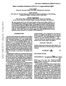
FIG. 1: Dilatation (left) and compression (right) phases in space correlation for isotropic turbulence. In a direct cascade scenario the flux vectors F (dashed arrows) are oriented towards the center of the sphere. Dilatation and compression (solid arrows) are additional effects which act respectively in the opposite or in the same direction as the flux vectors.

An illustration of dilation and compression effects in the space correlation is given in Fig. 1. In both cases, the flux vector F (dashed arrows) is oriented towards the center of the sphere (r = 0) since a direct cascade is expected. Dilatation and compression act additionally (solid arrows): in the first case, the effect is similar to a decrease of the local mean total energy transfer rate whereas in the second case it is similar to an increase of the local mean total energy transfer rate. The discussion may be extended to the entire inertial range (i.e. for larger values of r) when the (turbulent) Mach number is relatively high. In this case the analysis is focused on expression (14) for which we have already noted that a term like R − E is mainly negative. It is interesting to note that S(r) is composed of two types of term which are different by nature. First, there is the dilatation dominated by the smallest scales in the flow – the 7

shocklets – which mainly give a negative contribution with a fast variation [22]. Secondly, there is the correlation R − E which derives most of its contribution from relatively larger scales with a slower variation. This remark may lead to the assumption that both terms are relatively decorrelated [19]. Then S(r) may be simplified as (by using relation (4))    1 1 ¯ ∇ · u) δ(ρu) · δu + δρδe . S(r) ≃ − δ(∇ 4 2

(16)

The previous expression is not derived rigorously but it may give us some intuition about its contribution. For example, we may expect a power law dependence close to r 2/3 for the structure functions. Direct numerical simulations have never shown a scale dependence for the dilatation and we may expect that it behaves like a relatively small factor. Then S(r) will still modify ε as explained in the discussion above, however the power law dependence in r would be now slightly different. In conclusion and according to this simple analysis we see that compression effects (through the dilatation) will mainly impact the scaling law at the largest scales. Compressible spectrum. We may try to predict a power law spectrum for compressible turbulence. First, we note that several predictions have been made for the kinetic energy spectrum and also for the spectra associated with the solenoidal or the compressible part of the velocity [21]. We recall that although these decompositions are convenient for analytical developments, the associated energies are not inviscid invariants and the predictions are heuristic. For incompressible turbulence the situation is different because a prediction in k −5/3 for the kinetic energy spectrum may be proposed by applying a dimensional analysis directly on the 4/5s law [3]. Although it is not an exact prediction, the 4/5s law gives a stronger foundation to the energy spectrum for which a constant flux is expected. This remark was already noted in particular in recent 3D direct numerical simulations of isothermal turbulence where it is observed that the Kolmogorov scaling is not preserved for the spectra based only on the velocity fluctuations [15]. We shall derive a power law spectrum for compressible turbulence by applying a dimensional analysis on equation (11). Dimensionally, we may find εeff r ∼ ρu3 . By introducing the density-weighted fluid velocity, v ≡ ρ1/3 u, and following Kolmogorov we obtain 2/3

E v (k) ∼ εeff k −5/3 , where E v (k) is the spectrum associated to the variable v. Our prediction is compatible with the measurements recently made by direct numerical simulations [15] where the authors have noted that the exponent of the third-order velocity structure 8

function is close to one if the field used is v instead of u. (Note that two other scaling relations may be predicted like for the pressure term.) As explained by several authors [21] in compressible turbulence we do not expect a constant flux in the inertial range. Here, the same conclusion is reached since we are dealing with an effective mean energy transfer rate. More precisely if we expect a power law dependence in k for the effective transfer rate one arrives at the conclusion that a steeper power law spectrum may happen at the largest scales. According to relation (16) and the simple estimate, ρv 2 ∼ r 2/3 , we could have E v (k) ∼ k −19/9 . This prediction means that for a small prefactor in (16) one needs an extended inertial range to feel the compressible effects on the power spectrum. The scale at which the transition happens between −19/9 and −5/3 may be the sonic scale ks as proposed in [23] where such power laws were detected; in our case, a rough estimate gives ks ∼ h(∇ · u)/δui. Conclusion. The present work opens important perspectives to further understand the nature of compressible turbulence in the asymptotic limit of large Reynolds numbers with the possibility to extend the analysis to magnetized fluids with possibly other types of closures (e.g. polytropic gas), or to improve intermittency models by using the new relation – obtained by a statistical analysis at low order – as pivotal for a heuristic extension to statistical laws at higher order. We believe that astrophysics (e.g. interstellar turbulence) is one of the most important domain of application of the present work [10]. Acknowledgment. We acknowledge S. Boldyrev, A. Kritsuk and T. Passot for useful discussions.

[1] A.C. Newell and B. Rumpf, Annu. Rev. Fluid Mech. 43, 59 (2011); S. Galtier, Nonlin. Proc. Geophys. 16, 83 (2009). [2] A.N. Kolmogorov, Dokl. Akad. Nauk SSSR 32, 16 (1941); R.A. Antonia and P. Burattini, J. Fluid Mech. 550, 175 (2006). [3] U. Frisch, Turbulence: the legacy of A.N. Kolmogorov (Cambridge Univ. Press, Cambridge, 1995). [4] A.M. Yaglom, Dokl. Akad. Nauk SSSR 69, 743 (1949); H. Politano and A. Pouquet, Phys. Rev. E 57, R21 (1998); S. Galtier, Phys. Rev. E 77, R015302 (2008); S. Galtier, J. Geophys.

9

Res. 113, A01102 (2008). [5] S. Galtier, CRAS 12, 151 (2011). [6] V.E. Zakharov and R.Z. Sagdeev, Sov. Phys. 15, 439 (1970). [7] S. Chandrasekhar, Proc. Roy. Soc. A 210, 18 (1951). [8] O. Zeman, Phys. Fluid A 2, 178 (1990). [9] P. Sagaut and C. Cambon, Homogeneous Turbulence Dynamics (Cambridge Univ. Press, Cambridge, 2008). [10] T. Passot and E. Vazquez-Semadeni, Phys. Rev. E 58, 4501 (1998); B. G. Elmegreen and J. Scalo, Annu. Rev. Astron. Astrophys. 42, 211 (2004). [11] T. Passot, A. Pouquet and P. Woodward, Astron. Astrophys. 197, 228 (1988); S. Boldyrev, A. Nordlund and P. Padoan, Phys. Rev. Lett. 89, 031102 (2002). [12] J. Bec and K. Khanin, Phys. Rep. 447, 1 (2007); J.-P. Bouchaud, M. M´ezard and G. Parisi, Phys. Rev. E 52, 3656 (1995). [13] A.M. Polyakov, Phys. Rev. E 52, 6183 (1995). [14] S. Lee, S.K. Lele and P. Moin, Phys. Fluids A 3, 657 (1991); D.H. Porter, A. Pouquet and P.R. Woodward, Phys. Rev. Lett. 68, 3156 (1992); W. Schmidt, C. Federrath and R. Klessen, Phys. Rev. Lett. 101, 194505 (2008). [15] A. G. Kritsuk, M.L. Norman, P. Padoan and R. Wagner, Astrophys. J. 665, 416 (2007). [16] D. Porter, A. Pouquet and P.R. Woodward, Phys. Rev. E 66, 026301 (2002). ´ Mir, 2nd ed., Sov. Union, 1989). [17] L. Landau and E. Lifchitz, M´ecanique des fluides (Ed. [18] G.K. Batchelor, The theory of homogeneous turbulence (Cambridge Univ. Press, Cambridge, 1953). [19] H. Aluie, Phys. Rev. Lett. 106, 174502 (2011). [20] R.A. Antonia, M. Ould-Rouis, F. Anselmet and Y. Zhu, J. Fluid Mech. 332, 395 (1997). [21] J.E. Moyal, Proc. Cambridge Philos. Soc. 48, 329 (1952); B.B. Kadomtsev and V.I. Petviashvili, Sov. Phys. Dokl. 18, 115 (1973); S.S. Moiseev, V.I. Petviashvili, A.V. Toor and V.V. Yanovsky, Physica D 2, 218 (1981). [22] M.D. Smith, M.-M. Mac Low and J.M. Zuev, Astron. Astrophys. 356, 287 (2000). [23] C. Federrath et al., Astron. Astrophys. 512, A81 (2010).

10