Jul 28, 2017 - by numerous example setups. The test cases are provided as plain Python or. Octave/MATLAB script files for immediate replication. Contents.
Example Setups of Navier-Stokes Equations with Control and Observation: Spatial Discretization and Representation via Linear-quadratic Matrix Coefficients arXiv:1707.08711v1 [cs.MS] 27 Jul 2017
Maximilian Behr
Peter Benner
Jan Heiland
July 28, 2017
We provide spatial discretizations of nonlinear incompressible Navier-Stokes equations with inputs and outputs in the form of matrices ready to use in any numerical linear algebra package. We discuss the assembling of the system operators and the realization of boundary conditions and inputs and outputs. We describe the two benchmark problems driven cavity and cylinder wake and provide the corresponding data. The use of the data is illustrated by numerous example setups. The test cases are provided as plain Python or Octave/MATLAB script files for immediate replication.
Contents 1 Introduction
2
2 Spatial Discretization of Navier-Stokes Equations
3
3 Assembling the Linear Operators
4
4 Assembling of the Trilinear Form
4
5 Incorporation of Boundary Conditions 5.1 Dirichlet Boundary Conditions . . . . . . . . . . . . . . . . . . . . . . . . 5.2 Natural Boundary Conditions . . . . . . . . . . . . . . . . . . . . . . . . .
5 5 6
6 The Spatially Discretized System
7
7 Simulating the System 7.1 Steady-state Solutions . . . . . . . . . . . . . . . . . . . . . . . . . . . . .
7 8
1
7.2 7.3
Linearizations . . . . . . . . . . . . . . . . . . . . . . . . . . . . . . . . . . Time Integration . . . . . . . . . . . . . . . . . . . . . . . . . . . . . . . .
8 9
8 Setups 9 8.1 Lid Driven Cavity . . . . . . . . . . . . . . . . . . . . . . . . . . . . . . . 9 8.2 Cylinder Wake . . . . . . . . . . . . . . . . . . . . . . . . . . . . . . . . . 10 9 Modelling and Approximation of Control and Observation 9.1 Distributed Control and Observation . . . . . . . . . . . . . . . . . 9.2 Assembling of the Distributed Control and Observation Operators 9.3 Boundary Control . . . . . . . . . . . . . . . . . . . . . . . . . . . 9.4 Assembling of the Boundary Control Operator . . . . . . . . . . . .
. . . .
11 12 13 15 16
10 Control Setups 10.1 Driven Cavity with Distributed Control and Observation . . . . . . . . . . 10.2 Cylinder Wake with Distributed Control and Observation . . . . . . . . . 10.3 Cylinder Wake with Boundary Control . . . . . . . . . . . . . . . . . . . .
16 17 17 17
11 The 11.1 11.2 11.3
18 18 19 19
Data, Plotting, and Auxiliary The System Matrices Files . . Files for Visualizations . . . . Auxiliary Files . . . . . . . .
. . . .
. . . .
. . . .
Functions . . . . . . . . . . . . . . . . . . . . . . . . . . . . . . . . . . . . . . . . . . . . . . . . . . . . . . . . . . . . . . . . . . . . . . . . . . .
12 Numerical Examples 12.1 Cylinder Wake . . . . . . . . . . . . . . . . . . . . . . . . . . . 12.1.1 Steady State with Re=40 . . . . . . . . . . . . . . . . . . 12.1.2 Steady State with Re=40 with Boundary Control Impact 12.1.3 Transient Case with Re=90 . . . . . . . . . . . . . . . . . 12.1.4 Transient Case with Re=40 and Boundary Actuation . . 12.2 Driven Cavity . . . . . . . . . . . . . . . . . . . . . . . . . . . . 12.2.1 Steady State with Re=1200 . . . . . . . . . . . . . . . . 12.2.2 Transient Case with Re=800 and Distributed Actuation .
. . . . . . . .
. . . . . . . .
. . . . . . . .
. . . . . . . .
. . . . . . . .
19 19 20 20 20 23 23 23 25
. . . . . . . .
1 Introduction This work considers spatial discretizations of incompressible Navier-Stokes equations ∂v + (v · ∇)v − ∂t
1 Re ∆v
+ ∇p = f in (0, t) × Ω,
(1a)
∇ · v = 0 in (0, t) × Ω,
(1b)
with controls and observations, which we assume to be parametrized by the Reynolds number Re, posed on a bounded domain Ω ⊆ R2 for time t > 0, and equipped with an initial condition and boundary conditions.
2
This manuscript is accompanied by data that represents spatial discretizations of (1) in various flow setups. The modelling of the flow problems, the discretizations, and the data representation comes with the following features and advantages 1. The discretized nonlinearity is provided as an unfolded tensor H, that realizes H(v, v) as H · v ⊗ v. On the one hand side, this leads to a pure matrix representation. On the other hand, the tensor representation is directly accessible to recent developments of model reduction for bilinear quadratic systems. 1 2. The terms that are multiplied with Re are kept separate, so that simulations with different Reynolds numbers can be realized through a scaling of the corresponding matrices.
3. Nonhomogeneous boundary conditions are incorporated via a penalized Robin approach. This allows us to model the control action via an linear input operator that appears in the right hand side of the momentum equation (1a) as in the case of distributed control; cf. [2]. Altogether, these approaches provide a discrete representation of nonlinear Navier-Stokes equations with control and observations that can be readily used for simulations and system theoretical experiments not resorting to any finite element toolbox whatsoever. The manuscript is structured as follows. First, we explain how the system coefficient matrices of the semi-discrete Navier-Stokes equations are assembled and explain the basic usage of the matrices in simulations. Then, we introduce the test setups for simulation or control of imcompressible flows. In the last part, we document the data files and the setup and results of some example configurations. Code and Data Availability The source code and the data of the implementations used to compute the presented results is available from: doi:10.5281/zenodo.834940 under the MIT license.
Figure 1: Link to code and data.
2 Spatial Discretization of Navier-Stokes Equations We consider a general mixed finite element scheme to illustrate the derivation. For mathematical and practical details on finite element approximations of flows, see, e.g., [3, 4]. Let V and Q be the finite element space, namely finite-dimensional function spaces defined on a tesselation of Ω, for the velocity and the pressure spanned by nodal bases
3
like V = span{φi }ni=1
and Q = span{ψk }m k=1 ,
n, m ∈ N.
(2)
Thus, we look for approximations v and p to the velocity and pressure solutions of (1) that are linear combinations of the basis functions, namely v(t, x) =
n X
vj (t)φj (x) and p(t, x) =
j=1
m X
pk (t)ψk (x).
(3)
k=1
In what follows, we will often omit the time dependency of the coefficients and the space dependency of the basis functions. Also, we will freely identify the discrete functions v and p with their coefficient vectors v1 p1 p2 v2 v = . and p = . . . .. vn pm defined through the expansion in (3).
3 Assembling the Linear Operators For the finite element spaces (2), we assemble the finite dimensional approximations A and J to the diffusion and divergence operators ∆ and ∇· in the standard way: �Z � �Z � A= ∇φi : ∇φj dx ∈ Rn×n and J = ψk ∇ · φj dx ∈ Rn×n , i=1,...,n j=1,...,n
Ω
k=1,...,m j=1,...,n
Ω
(4) where : stands for the Frobenius inner product. The mass matrix M and the right hand side f are assembled as follows: �Z � �Z � n×n M= φi · φj dx ∈R and fn = φi · f dx ∈ Rn×1 . Ω
i=1,...,n j=1,...,n
Ω
(5)
i=1,...,n
By now, we haven’t taken into account the boundary conditions. This we will discuss in Section 5.
4 Assembling of the Trilinear Form Consider two discrete velocities v =
n P
vj φj and w =
j=1
n P
wk φk with coefficient vectors
k=1
v and w and the resulting convective term (v · ∇)w =
n X n X j=1 k=1
4
vj wk (φj · ∇)φk .
Testing this relation against the i-th basis function gives the relation n X n X j=1 k=1
Z ((φj · ∇)φk ) · φi dx = Hi (v ⊗ w),
v j wk Ω
2
with the Kronecker product ⊗ : Rn × Rn → Rn and where �R � 2 Hi := Ω (φj · ∇)φk · φi dx j=1,...,n; k=1,...,n ∈ R1×n
(6)
Thus, the discrete approximation of the convection operator v 7→ (v · ∇)v is given as H1 2 .. (7) H : v 7→ H(v ⊗ v), where H = . ∈ Rn×n Hn and Hi is as defined in (6).
5 Incorporation of Boundary Conditions We now explain how boundary conditions are treated in general and for the trilinear form in particular.
5.1 Dirichlet Boundary Conditions To begin with, we assume that we only have Dirichlet conditions for the velocity. This means that the value of v at the boundary is known and, since we consider nodal bases, also the values of the coefficients of the discretized velocities associated with nodes at the boundary are known. In the theory of weak solutions, the test space is chosen to have a zero trace at the Dirichlet boundary. In practice, the basis functions φi that are associated with a node at a Dirichlet boundary, are left out when assembling the coefficient matrices like in (4) and (5). Often it is more convenient to assemble the whole matrices and remove the lines corresponding to the boundary in a second step. Let IΓ be the set of indices associated with the Dirichlet boundary nodes and let II be the set that contains the indices of all other nodes, i.e. the nodes in the inner or at the boundary where Neumann conditions are posed. Assume that the entries of the solution vector are sorted such that � � � � v 0 ¯I + v ¯ Γ := I + v=v , (8) 0 vΓ where vI and vΓ are the vectors of coefficients associated with II and IΓ . Let [·]I denote the operation of restricting a matrix or vector to the inner nodes with respect to degrees of freedom (columns) and the posed conditions (rows). For example,
5
assume that A is assembled without considering boundary conditions. Then, we resolve given Dirichlet boundary conditions via the relation [Av]I = [A]I vI + [A¯ vΓ ]I .
(9)
We will use the abbreviation AI := [A]I . For the quadratic term, we first compute ¯ I ) + H(¯ ¯ Γ ) + H(¯ ¯ I ) + H(¯ ¯ Γ ). H(v ⊗ v) = H(¯ vI ⊗ v vI ⊗ v vΓ ⊗ v vΓ ⊗ v ¯ I and v ¯ Γ , it holds that Because of the zero entries in v ¯ Γ )]I , [H(v ⊗ v)]I = HI (vI ⊗ vI ) + [L1 (¯ vΓ )]I vI + [L2 (¯ vΓ )]I vI + [H(¯ vΓ ⊗ v
(10)
where L1 (¯ vΓ ) =
X
Z ((φj · ∇)φk ) · φi dx
[vΓ ]k Ω
k∈IΓ
(11a)
.
(11b)
i=1,...,n j=1,...,n
L2 (¯ vΓ ) =
,
X
Z ((φk · ∇)φj ) · φi dx
[vΓ ]k Ω
k∈IΓ
i=1,...,n j=1,...,n
Thus, the consideration of Dirichlet boundary conditions in the quadratic formulation can be done as follows 1. Assemble H = HI like in (7) for the inner nodes both in test and trial space. ¯ Γ as convection velocity 2. Assemble the linearized convection matrix L(¯ vΓ ) with v like L1 (¯ vΓ ) and L2 (¯ vΓ ) in (11) and restrict it to the inner nodes. ¯ Γ ) to the source term via 3. Assemble the contribution H(¯ vΓ ⊗ v
¯Γ) = H(¯ vΓ ⊗ v
X X
Z ((φj · ∇)φk ) · φi dx
[vΓ ]j [vΓ ]k Ω
j∈IΓ k∈IΓ
i=1,...,n
and restrict it to the inner nodes. As the result, one has the coefficient for vI ⊗ vI , an additional coefficient matrix for vI , and a correction for the source term.
5.2 Natural Boundary Conditions Boundary conditions that contain the normal derivative of v are often called natural boundary condtions since they like naturally are resolved in the finite element discretization. In view of assembling the coefficients, nodes associated with natural boundary are
6
simply treated like inner nodes. However, one has to consider additional source terms, that derive from the partial integration that led to the forms in (4). Let ΓN denote the part of the boundary where boundary conditions other than of Dirichlet type are applied. Then the additional source term is assembled as �Z � �Z � ∂v gn = = (p~n − ν ) · φi dx g · φi dx , (12) ∂~n ΓN ΓN i=1,...,n i=1,...,n where ~n is the outward normal vector. We will frequently employ do-nothing conditions at the outflow boundary, i.e. we set p~n − ν
∂v = 0, ∂~n
on ΓN ,
(13)
so that gn is just zero.
6 The Spatially Discretized System We consider the Navier-Stokes equations ∂v − ∂t
1 Re ∆v
+ (v · ∇)v + ∇p = fn , ∇ · v = 0,
(14a) (14b)
on the domain Ω with Dirichlet or do-nothing boundary conditions that we write as γv = vΓ .
(14c)
With the splitting of the velocity ansatz space into inner and boundary nodes as defined in (8), with the convention (9), and with the formula for the convective term (10), a standard finite element discretization of (14) for the velocity at the inner nodes vI and the discrete pressure p can be written as d vI + HI (vI ⊗ vI ) + [L1 (¯ vΓ ) + L2 (¯ vΓ ) + MI dt
1 Re A]I vI
− JIT p = [fn ]I − [gn ]I − ¯ Γ ]I . JI vI = −[J v
1 vΓ ]I Re [A¯
¯ Γ )]I , − [H(¯ vΓ ⊗ v (15a)
(15b)
¯ Γ is defined through (14c), and, thus, we can define system (15) For a given setup, v completely by means of the matrices and vectors up to a scaling of A and fv_diff by
1 Re .
7 Simulating the System Once one has the coefficients listed in Table 1 at hand, the implementation of a simulation can be done in any numerical linear algebra package. To illustrate the usage, we address a few important points of a simulation.
7
M A H L1 L2 J J.T
↔ ↔ ↔ ↔ ↔ ↔ ↔
MI AI HI [L1 (¯ vΓ )]I [L2 (¯ vΓ )]I JI JIT
fv gv fv_diff fv_conv fp_div
and
↔ ↔ ↔ ↔ ↔
[fn ]I [gn ]I [A¯ vΓ ]I [N (¯ vΓ )¯ vΓ ] I [J(¯ vΓ )]I
Table 1: Parameters defining the spatially discretized Navier-Stokes equations (15).
7.1 Steady-state Solutions For a Reynolds number RE, the steady-state Stokes solution [v, p] is defined through � � � � � � 1./RE*A -J.T v fv - 1./RE*fv_diff * != (16) J 0 p -fp_div and the steady-state Navier-Stokes solution is given as the solution of � � � � � � fv - H*kron(v, v)- 1./RE*fv_diff - fv_conv v 1./RE*A+L1+L2 -J.T , != * -fp_div p J 0 where != means that a solver has to be applied and where kron is the function that computes the Kronecker product. Note that v represents the velocity solution only at the inner nodes, while the values of the boundary nodes are defined by the boundary conditions.
7.2 Linearizations We consider linearizations as they occur in the modelling of optimal control systems or during the numerical solution of the nonlinear state equations. In the nonlinear setting the convection is modelled through L1 * v + L2 * v + H * kron (v , v ) + fv_conv If a is a linearization point that in particular fulfills the boundary conditions and if a is its approximation, then the Oseen or Picard linearization (u · ∇)u ← (a · ∇)u is realized as H * kron (a , v ) + L1 * v + L2 * a + fv_conv and the Newton linearization (u · ∇)u ← (a · ∇)u + (u · ∇)a − (a · ∇)a as H * kron (a , v ) + H * kron (v , a ) - H * kron (a , a ) + L1 * v + L2 * v + fv_conv In the frequent case, that one decomposes v != vs + vd, where vs is the steady-state Navier-Stokes solution, the linearized system for the difference state vd to be solved reads
8
M * vd . dt + A * vd + H * kron ( vs , vd ) + H * kron ( vd , vs ) - J . T * p != 0 # and , simultaneously , J * vd != 0 where vd.dt denotes the time derivative. Note that, because the difference state is zero at the boundary, in particular the terms L1+L2 and f_conv do not appear. The matrices H1 and H2 representing the linear functions H*kron(a, v) =: H1*v and H*kron(v, a) =: H2*v can be computed columnwise: H1 = [ H * kron ( e_i , a ) for i in range ( Nv )] H2 = [ H * kron (a , e_i ) for i in range ( Nv )] where a[i] is the i-th component of a and e_i is the i-th unit basis vector.
7.3 Time Integration Assume that the current velocity approximation v_old is given. Then one can apply the implicit-explicit (IMEX) Euler scheme to advance the velocity by a time step of size dt by solving
�
� � � M + dt*(A+L1+L2) -dt*J.T v_new * != J 0 p � � M*v_old + dt*(fv - H*kron(v_old, v_old)- fv_diff - fv_conv) . -fp_div
8 Setups We describe the setups for which the coefficient matrices can be downloaded. For all considered setups we describe the geometrical properties, the boundary conditions. The provided matrices are obtained by finite element discretizations as provided by FEniCS [6]. Depending on the geometry, we use uniform and nonuniform grids of different coarseness. As finite element pair we choose Taylor-Hood P2 −P1 finite elements [10].
8.1 Lid Driven Cavity The two-dimensional driven cavity is a well investigated and common benchmark problem [8]. As the model, one considers the incompressible Navier-Stokes equations on a square with homogeneous Dirichlet boundary conditions for the velocity except from the upper boundary Γ0 – the lid – where the tangential velocity component is set to 1. In the setup of the regularized driven cavity the tangential velocity set to smoothly approach
9
1
1
Γ0
Ωo
0.5 0.3 0.2 0
x1
x1
0.7 0.5
Ωc 0
0.4
0.6
1
0
0
x0
0.5
1
x0
Figure 2: Illustration of the velocity magnitude of the driven cavity problem and the domain of control and observation Ωc = [0.4, 0.6] × [0.2, 0.3] and Ωo = [0.45, 0.55] × [0.5, 0.7]. The second plot shows a triangulation of the domain for N=10. zero towards the edges in order to comply with the zero conditions on the other walls. The regularized and standard driven cavity is a test problem of the Octave/MATLAB FE package IFISS [9]. We consider the non regularized driven cavity on the unit square Ω = (0, 1) × (0, 1) and its boundary Γ with boundary conditions ( v = [1, 0]T , on Γ0 , γv : v = [0, 0]T , elsewhere, cf. Fig. 2. For the spatial discretization, we use a uniform grid as illustrated in Fig. 2 with a parameter N that describes the number of segments that one boundary is divided into. Note that for flow setups with only Dirichlet boundary conditions for the velocity, like the driven cavity, the pressure is defined up to a constant. In the numerical approximation this leads to a rank deficiency of the divergence and the gradient matrices J and JT. For iterative schemes this does not pose a problem. However, in order to have the coefficient matrix in (16) invertible, one can pin the pressure to zero at one node of the discretization by simply removing the corresponding row and column of J and JT.
8.2 Cylinder Wake We consider the two dimensional wake of a cylinder which is a popular flow benchmark problem, a subject for simulations, and a test field for flow control [11, 7, 1]. The computational domain is as depicted in Fig. 3.
10
0.41
Γ0 x1
Γ1
0
0
2.2
x0
x1
0.41 0.25
Ωc
0.15 0
0
0.2 0.32
Ωo
0.6 0.7
2.2
x0
Figure 3: Illustration of geometrical setup including the domains of distributed control and observation and of the velocity magnitude for the cylinder wake. We consider the incompressible Navier-Stokes equations on the domain as illustrated in Fig. 3 with boundary Γ with boundary conditions as follows, at the inflow Γ0 we prescribe a parabolic velocity profile through the function g(s) = 4 1 −
s � s . 0.41 0.41
We impose do-nothing conditions, cf. (13), at the outflow Γ1 and no-slip, i.e. zero Dirichlet conditions, at the upper and the lower wall of the channel and at the cylinder periphery. T v = [g(x1 ), 0] , on Γ0 , 1 ∂v T γ(v, p) : p~n − Re on Γ1 , ∂~ n = [0, 0] , T v = [0, 0] , elsewhere on the boundary.
9 Modelling and Approximation of Control and Observation In flow control, one tries to act on the flow in such a way that certain flow pattern are stabilized or enforced by means of actuators. Also, sensors are used to monitor the process and to provide necessary information for the actuation. For the simulation, actuation and measuring are modelled through input and output operators B and C and corresponding spaces for the input and output signals u and y that are included in the equations as follows:
11
∂v + (v · ∇)v − ∂t
1 Re ∆v
+ ∇p = f + Bu,
(17a)
∇ · v = 0,
(17b)
y = C(v, p).
(17c)
Distributed control, where the control acts as a volume force distributed in a domain of control, is hardly realizable in practice. Nevertheless, we provide models for distributed control, because the modelling and spatial discretization naturally leads to a standard state-space system, which is the basis for typical control or model reduction algorithms. Boundary control through Dirichlet boundary conditions for the velocity, which is the setup for many flow control problems, does not simply lead to a standard state space representation, cf. [2]. We provide boundary control models in state space form by means of Robin approximations of the Dirichlet boundary conditions.
9.1 Distributed Control and Observation We define input and output state spaces U and Y as subspaces of L2 ([0, 1]). Let Ω be the computational domain and Ωc = [xc0,min , xc0,max ] × [xc1,min , xc1,max ] a rectangular subdomain where the control acts. We define the input operator B : U × U → [L2 (Ω)]2 such that the control acts distributed in the domain of control Ωc with two spatial components. In order to save some degrees of freedom, we assume that Bu is constant in one spatial direction – say x0 . Concretely, for U := L2 (0, T ; U × U ) we define the B : U → L2 (0, T ; L2 (Ω; R2 )) via ( u(t; θ(x1 )), for (x0 , x1 ) ∈ Ωc , Bu(t; x0 , x1 ) = (18) T [0, 0] , elsewhere, for u ∈ U and with the affine linear function θc mapping the x1 -extension of Ωc , [xc1,min , xc1,max ], onto [0, 1]. Note that the roles of x0 and x1 can be interchanged depending on the setup. The output operator PY Cv : L2 (0, T ; L2 (Ω; Rs ) → L2 (0, T ; Y × Y ) for the velocity is defined as follows 1. For v(t) ∈ L2 (Ω, R2 ) compute Cv v(t) ∈ L2 (0, 1; R2 ) through Cv v(t)(η) =
1 xo0,max −xo0,min
Z
xo0,max
xo0,min
v(t; x0 , θo (η)) dx0 ,
(19)
which, basically, is the velocity in the domain of observation Ωo averaged in x0 direction. Here, θo is an affine linear mapping adjusting [0, 1] to [xo1,min , xo1,max ].
12
2. Define the corresponding discrete signal y(t) ∈ L2 (0, T ; Y × Y ) as y(t) = PY Cv v(t), where PY : [L2 (0, 1)]2 → Y × Y is the L2 -orthogonal projection. Namely, for a rectangular domain of observation Ωo = [xo0,min , xo0,max ] × [xo1,min , xo1,max ], for Y := L2 (0, T ; Y × Y ), and for a v ∈ L2 (0, T ; L2 (Ω; R2 )), we define the observation operator Cv : v 7→ y ∈ Y via As a pressure-based output we take the average pressure in a subdomain Ωp = [xp0,min , xp0,max ] × [xp1,min , xp1,max ], i.e.
1 yp (t) = Cp p(t) := |Ωp |
Z p(t, x)dx
(20)
Ωp
evaluated in the corresponding finite element space.
9.2 Assembling of the Distributed Control and Observation Operators To setup a discrete representation of the input operator B, we impose several assumptions on the space-time structure of the input signals. Firstly, for a given Nu ∈ 2N, we choose the signal state space U × U as U0 ⊕ U1 , where U0 := span{~νl }l=1,...,Nu /2 and U1 := span{~νl }l=Nu /2+1,...,Nu , where � � 0 , for l = 1, . . . , Nu /2 and ~νl := νl
� � ν ~νl := l , 0
for l = Nu /2 + 1, . . . , Nu , (21)
with νl being the hierarchical piecewise linear hat functions illustrated in Figure 4. 1
1
1
0.5
0.5
0.5
0
0 0
0.5 ξ
1
0 0
0.5 ξ
1
0
0.5 ξ
1
Figure 4: Three levels of a hierarchical basis for piecewise linear functions for nested L2 (0, 1)-subspaces. Note that by defining U0 and U1 with only one spatial coordinate ξ, we anticipate that the input is to be defined depending only on one spatial coordinate, cf. (18), and note that bases of subspaces of L2 (0, 1) other than shown in Figure 4 can be used.
13
Secondly, we assume that the time and space component in the chosen discrete input space are separated, i.e., that we can write the inputs as u(t; ξ) =
Nu X
sl (t)~νl (ξ).
(22)
l=1
With u defined as (22) and the input to the system Bu as defined in (18) discretized like the right hand side as in (5), the discrete input operator B ∈ RNu → Rn , that maps the vector u = [s1 , . . . , sNu ]T of control coefficients, cf. (22), onto the control action Bu is defined as �Z
� φi : B~νl dx
B=
.
Ω
(23)
i=1,··· ,n; l=1,··· ,Nu
For the output space for the velocity measurements, given q ∈ 2N, we define Y × Y = Y0 ⊕ Y1 similar to U × U with basis functions for both spatial components as in (21). As basis functions we use q piecewise linear hat functions defined on [0, 1] partitioned into q/2 − 1 equidistant segments. From the space-time separated ansatz for the discrete velocity (3) and from the definition of the output operator in (20) it follows that the measured output will always be of the form PY Cv v(t)(η) =
n X
vj (t)PY Cv φj (η).
j=1
Since for every j = 1, · · · , n, the term PY Cv φj is in Y × Y and, thus, can be expanded in the basis (21), the measurement from the discrete velocity can be written as PY Cv v(t)(η) =
q X
yk (t)~νl (η),
(24)
l=1
with a unique vector of coefficients y := [y1 , · · · , yq ]T . These coefficients are obtained through the discrete approximation Cv to PY Cv that maps the coefficient vector v of the velocity approximation onto y and that is defined through Cv =
M−1 Y
�Z
1
� ~νl (η) : Cv φj (η) dη
0
.
(25)
l=1,··· ,q; j=1,··· ,n
This assembling is basically taking the output for all basis functions, testing them against the basis functions of Y × the obtained matrix by the inverse of hRY , and premultiplying i 1 the mass matrix MY := 0 ~νl (η) : ~νk (η) dη . k,l=1,··· ,q
The pressure based output as defined in (20) only depends on time, i.e. Cp : L2 (0, T ; Rm ) → L2 (0, T ). Thus, the discrete representation Cp of Cp that maps the coefficient vector p of a discrete pressure p, cf. (3), onto Cp p ∈ L2 (0, T ) is defined through Cp = [Cp ψk ];k=1,··· ,m .
14
(26)
B Cv Cp
↔ ↔ ↔
[B]I [Cv ]I Cp
and
My Mu
↔ ↔
MY MU
Table 2: Parameters defining the discrete input and output operators and the mass matrices of the signal state spaces. Depending on the setup, in the provided data files, the discrete input and output operators appear as listed in Table 2. In B, the first Nu /2 columns are associated with the control in x0 direction and the last Nu /2 columns with control in x1 direction. Thus, to vary the number of control parameters one may discard a control direction or, thanks to the hierarchy of the basis functions, only use, e.g., the first three columns. Similarly, in C the first q/2 rows correspond to the x0 component of the output, while the last q/2 rows correspond to the x1 component. To reduce the output dimension, one may also discard one component. Also one can discard single degrees of freedom in the output space. Note, however, that the basis in the output space is not hierarchical but the standard hat function basis.
9.3 Boundary Control A common case of boundary control of a flow is defining a time-varying velocity profile on a part of the boundary. This models, for example, a valve at the peripherie where one can inject a jet into the flow or exhaust certain amounts of the fluid. For illustration, we assume that such a control takes places at a single part Γc of the boundary Γ and that we have constant Dirichlet or do-nothing conditions elsewhere. The generalization to more controlled segments of the boundary and to other boundary conditions elsewhere is straight forward. So assume that the control action is given as v(t) Γc = u(t).
(27)
One may enforce the Dirichlet conditions by simply setting the values of the discrete approximations at the boundary. However, this leads to the appearance of u, ˙ cf. [2]. Therefore, we relax the Dirichlet to Robin conditions and approximate (27) via ∂v u(t) ≈ v(t) Γc + α(p~n − ν ) Γc , ∂~n
(28)
with a penalization parameter α that is intended to go to zero. This approximation of the Dirichlet control has been investigated in the context of optimal control of Navier–Stokes equations in [5].
15
Bbc Abc
↔ ↔
[Bbc ]I [Abc ]I
Table 3: The linear operators realizing the boundary control through the Robin relaxation with α = 1.
9.4 Assembling of the Boundary Control Operator We assume that u is given as a sum ofP spatial shape functions with time dependent u coefficients, i.e. u has the form u(x, t) = N l=1 gl (x)ul (t). ∂v 1 1 Rearranging (28) to p~n − ν ∂~ n Γc ≈ α u(t) − α v(t) Γc , the control is numerically realized through the term fN , cf. (12), which gives the linear coefficient �Z � 1 Abc = φi : φj dx , (29) α ΓN i,j=1,...,n and the source term, Bbc u, where u := [u1 , . . . , uNu ]T and �Z � 1 φi : gl dx . Bbc = α ΓN i=1,...,n; l=1,...,Nu Depending on the setup, in the provided data files, the discrete boundary control operators appear as listed in Table 3. There also α is set to 1 so that different penalization parameter values can be realized through scaling Abc and Bbc correspondingly. Note, that there is no constant contribution of other Dirichlet boundary values through ¯ Γ , cf. (9). A contribution may occur where a Dirichlet and a Robin node share some Abc v support on ΓN (cf. (29)) which can only happen where Dirichlet and control boundaries meet. However, in the considered setups the control boundaries are in the neighborhood of zero Dirichlet so that the possible contribution would be zeroed out by the prescribed node value. If one considers Robin control, the set II , cf. (8), will also contain the Robin nodes as if they were inner nodes. Accordingly, these nodes are also solved for in the process of the simulations and they simply integrated as inner nodes in the assembling of the linear and nonlinear operators; cf. Sections 3 and 4.
10 Control Setups We describe the particular setups that include control and observation.
16
10.1 Driven Cavity with Distributed Control and Observation We consider the test case of the lid driven cavity described in Section 8.1 and add distributed control and observation that are defined and assembled as described in Section 9. Specifically, we define the domain of control and observation of the velocity as Ωc := [0.4, 0.6] × [0.2, 0.3] and Ωo := [0.45, 0.55] × [0.5, 0.7], see Figure 2. The pressure is observed in Ωp := [0.45, 0.55] × [0.7, 0.8]. Recall that the input and the velocity output were modelled with only one dimensional space dependencies, cf. (18) and (19). For the driven cavity the spatial components of the signal are modelled as follows
input output
x0 -direction space-varying constant (averaged)
x1 -direction constant space-varying
Table 4: Spatial components of the input and velocity output signals for the distributed control of the driven cavity problem.
10.2 Cylinder Wake with Distributed Control and Observation The test case of the cylinder wake is described in Section 8.2. Again, we add distributed control and observation as defined in Section 9. Specifically, we define the domain of control and observation of the velocity as Ωc := [0.27, 0.32] × [0.15, 0.25] and Ωo := [0.6, 0.7] × [0.15, 0.25], see Figure 3. The pressure is observed in Ωp := [0.6, 0.64] × [0.18, 0.22]. Recall that the input and the velocity output were modelled with only one dimensional space dependencies, cf. (18) and (19). For the cylinder wake, the spatial components of the signal are modelled as follows
input output
x0 -direction constant constant (averaged)
x1 -direction space-varying space-varying
Table 5: Spatial components of the input and velocity output signals for the distributed control of the driven cavity problem.
10.3 Cylinder Wake with Boundary Control The setup of the simulation and of the output definition is the same as described in Section 10.2. For the input we define and assemble a penalized Robin scheme as explained
17
Figure 5: Illustration of the control locations on the cylinder periphery. in Section 9.4. Specifically, we define the control through injection and suction at outlets Γc1 , Γc2 centered at the cylinder periphery at ±π/3 occupying π/6 of the circumference. Then, we prescribe Dirichlet conditions for the velocity v = n1 g1 (x)u1 (t),
v = n2 g2 (x)u2 (t),
at Γc1 and Γc2 , where n1/2 are the vectors that are normal to the outlets in their center and that point into the domain, where u1/2 are the magnitudes of the controls, and where g1/2 are the shape functions that parametrize the segments Γc1 /Γc2 via s ∈ [0, 1] and that return the value of 1 − 0.5(1 + sin((2s + 0.5)π)), thus realizing a shape function that is 1 in the center of the control outlets and that smoothly extends to the zero no-slip conditions at the adjacent boundaries.
11 The Data, Plotting, and Auxiliary Functions 11.1 The System Matrices Files The provided data, see Table 1, are vectors and sparse matrices stored as .mat files in the MATLAB 6 version. The naming of the data is as PROBLEMNAME__mats__NV*XX*_Re1[_bccontrol_palpha1].mat where • PROBLEMNAME={cylinderwake,drivencavity}, • *XX* denotes the size of the system, namely the dimension of the velocity approximation space, and • [_bccontrol_palpha1] is present, if boundary control is realized.
18
drivencavity N=10 ↔ NV=722 N=20 ↔ NV=3042 N=30 ↔ NV=6962
cylinderwake N=1 ↔ NV=5812 N=2 ↔ NV=9356 N=3 ↔ NV=19468
cylinderwake_bccontrol N=1 ↔ NV=5824 N=2 ↔ NV=9384 N=3 ↔ NV=19512
Table 6: Relation of the mesh parameters N and the discretization parameter NV for the considered problems and the provided data.
11.2 Files for Visualizations Visualization is done through writing the values of the pressure or velocity approximation to .vtu files that can be viewed in Paraview. For this there are json files that, among others, contains the geometrical information of the mesh and the map of the coordinates of the approximating vectors to the mesh vertices and that are named as visualization_PROBLEMNAME_N*XX*.jsn with PROBLEMNAME as above and *XX* standing for the discretization level. Note that N is different from NV used for the naming of the system matrices, since on a given mesh topology one can define approximations of, e.g., different degrees of freedom. For the provided data, the relations between mesh parameters N and approximation scheme parameters NV are listed in Table 6.
11.3 Auxiliary Files The data comes with two software modules, namely conv_tensor_utils that provides functionality for linearization and memory-efficient evaluation of the nonlinearity and visualization_utils that assists in writing output files for rendering in Paraview.
12 Numerical Examples We illustrate the use of the data in some example setups.
12.1 Cylinder Wake In this section, we consider example setups for the cylinder wake as described in Sections 8.2, 10.2, and 10.3.
19
12.1.1 Steady State with Re=40 Setup: cylinderwake Steady state simulation Reynolds number: Re=40 Grid: N=1
Simulation results: |v|: Figure 6 p: Figure 6
To replicate this simulation run cylinderwake_steadystate.{m,py} 12.1.2 Steady State with Re=40 with Boundary Control Impact Setup: cylinderwake Steady state simulation Reynolds number: Re=40 Grid: N=2 Robin-Penalization: palpha=1e-3 Input: uvec=[1,-1].T
Simulation results: |v|: Figure 7 p: Figure 7
To replicate this simulation run cylinderwake_steadystate_bccontrol.{m,py} 12.1.3 Transient Case with Re=90 Setup: cylinderwake Transient simulation with IMEX-Euler Reynolds number: Re=90 Grid: N=3 Time grid: t0, tE, Nts = 0., 4., 2**11 Initial value: Stokes solution
Simulation results: |v[t=tE]|: Figure p[t=tE]: Figure C*v: Figure C*p: Figure
To replicate this simulation run cylinderwake_tdp_vout_pout.{m,py}
20
8 8 9 9
Figure 6: Illustration of the velocity magnitude and pressure field for the setup described in Section 12.1.1
Figure 7: Illustration of the velocity magnitude and pressure field for the setup described in Section 12.1.2
21
Figure 8: Illustration of the velocity magnitude and pressure field at t=4.0 for the setup described in Section 12.1.3
·10−4 2 0.00025 0.00020 0.00015 0.00010 0.00005 0.00000
1
0
1
2
3
4
0
0
1
2
3
4
Figure 9: Illustration of the velocity and pressure output for the setup described in Section 12.1.3
22
12.1.4 Transient Case with Re=40 and Boundary Actuation Setup: cylinderwake Transient simulation with IMEX-Euler Reynolds number: Re=40 Grid: N=2 Time grid: t0, tE, Nts = 0., 6., 2**10 Initial value: Stokes solution Robin-Penalization: palpha=1e-3 Input frequency: omega=3*Pi/(tE-t0) Input: uvec=sin(omega*t)*[1,-1].T
Simulation results: C*v: Figure 10 C*p: Figure 10
To replicate this simulation run cylinderwake_tdp_pout_vout_bccontrol.{m,py}
12.2 Driven Cavity In this section, we consider example setups for the driven cavity as described in Sections 8.1 and 10.1. 12.2.1 Steady State with Re=1200 Setup: drivencavity Steady state simulation Reynolds number: Re=1200 Grid: N=30
Simulation results: |v|: Figure 11 p: Figure 11
To replicate this simulation run drivencavity_steadystate.{m,py}
23
0.0026 0.0024 0.0022 0.0020 0.0018 0.0016 0.0014 0.0012
·10−3 2.5 2 1.5 0
2
4
6
0
2
4
6
Figure 10: Illustration of the velocity and pressure output for the setup described in Section 12.1.4
Figure 11: Illustration of the velocity magnitude and pressure field for the setup described in Section 12.2.1
24
12.2.2 Transient Case with Re=800 and Distributed Actuation Setup: drivencavity Transient simulation with IMEX-Euler Reynolds number: Re=800 Grid: N=20 Time grid: t0, tE, Nts = 0., 20., 2**12 Initial value: Stokes solution Input frequency: omega=4*Pi/(tE-t0) Input: uvec=[sin(omega*t), cos(omega*t)].T
Simulation results: v(tk): Figure 12 C*v: Figure 13 C*p: Figure 13
To replicate this simulation run drivencavity_tdp_pout_vout_distcontrol.{m,py}
References [1] P. Benner and J. Heiland. LQG-Balanced Truncation low-order controller for stabilization of laminar flows. In R. King, editor, Active Flow and Combustion Control 2014, volume 127 of Notes on Numerical Fluid Mechanics and Multidisciplinary Design, pages 365–379. Springer, Berlin, 2015. [2] P. Benner and J. Heiland. Time-dependent Dirichlet conditions in finite element discretizations. ScienceOpen Research, 2015. [3] H. C. Elman, D. J. Silvester, and A. J. Wathen. Finite Elements and Fast Iterative Solvers: With Applications in Incompressible Fluid Dynamics. Oxford University Press, Oxford, UK, 2005. [4] P. M. Gresho and R. L. Sani. Incompressible Flow and the Finite Element Method. Vol. 2: Isothermal Laminar Flow. Wiley, Chichester, UK, 2000. [5] L. S. Hou and S. S. Ravindran. Numerical approximation of optimal flow control problems by a penalty method: Error estimates and numerical results. SIAM J. Sci. Comput., 20(5):1753–1777, 1999. [6] A. Logg, K. B. Ølgaard, M. E. Rognes, and G. N. Wells. FFC: the FEniCS form compiler. In Automated Solution of Differential Equations by the Finite Element Method, pages 227–238. Springer, Berlin, Germany, 2012. [7] B. R. Noack, K. Afanasiev, M. Morzyński, G. Tadmor, and F. Thiele. A hierarchy of low-dimensional models for the transient and post-transient cylinder wake. Journal of Fluid Mechanics, 497:335–363, 2003. [8] P. N. Shankar and M. D. Deshpande. Fluid mechanics in the driven cavity. In J. L. e. a. Lumley, editor, Annual review of fluid mechanics, volume 32, pages 93–136. Annual Reviews Inc., 2000.
25
Figure 12: Illustration of the velocity magnitude field for the setup described in Section 12.2.2 at t=0.0, 0.5, 1.0, 1.5, 2.0, 2.5, 3.0, 3.5, 4.0.
·10−4 0.4
−2
0.2 −4
0 −0.2
−6 0
5
10
15
20
−0.4
0
5
10
15
20
Figure 13: Illustration of the velocity and pressure output for the setup described in Section 12.2.2
26
[9] D. Silvester, H. Elman, and A. Ramage. and Iterative Solver Software (IFISS) version http://www.manchester.ac.uk/ifiss/.
Incompressible 3.3, October
Flow 2013.
[10] C. Taylor and P. Hood. A numerical solution of the Navier-Stokes equations using the finite element technique. Internat. J. Comput. & Fluids, 1(1):73–100, 1973. [11] C. H. K. Williamson. Vortex dynamics in the cylinder wake. Fluid Mechanics, 28(1):477–539, 1996.
27
Annual Review of