description and our results for ASIC1 are reasonably close to those obtained with the full self-consistent procedure SIC-. B3LYP. This is an interesting result, ...
THE JOURNAL OF CHEMICAL PHYSICS 127, 034112 共2007兲
Exchange parameters from approximate self-interaction correction scheme A. Akande and S. Sanvito School of Physics and CRANN, Trinity College, Dublin 2, Ireland
共Received 2 April 2007; accepted 29 May 2007; published online 20 July 2007兲 The approximate atomic self-interaction correction 共ASIC兲 method to density functional theory is put to the test by calculating the exchange interaction for a number of prototypical materials, critical to local exchange and correlation functionals. ASIC total energy calculations are mapped onto a Heisenberg pairwise interaction and the exchange constants J are compared to those obtained with other methods. In general the ASIC scheme drastically improves the band structure, which for almost all the cases investigated resemble closely available photoemission data. In contrast the results for the exchange parameters are less satisfactory. Although ASIC performs reasonably well for systems where the magnetism originates from half-filled bands, it suffers from similar problems than those of local density approximation for other situations. In particular, the exchange constants are still overestimated. This reflects a subtle interplay between exchange and correlation energy, not captured by the ASIC. © 2007 American Institute of Physics. 关DOI: 10.1063/1.2751165兴 I. INTRODUCTION
Theoretical studies based on density functional theory1,2 共DFT兲 have given remarkable insights into the electronic and magnetic properties of both molecules and solids.3 In particular, a number of these studies attempt to quantitatively describe the magnetic interaction in a broad range of systems including transition metals,4 hypothetical atomic chains,5,6 ionic solids,7–9 transition metal oxides,10,11 and transition metal polynuclear complexes.12–14 DFT uses an effective single-particle picture where spin symmetry is generally broken. For this reason exchange parameters J are conventionally extracted by using a mapping procedure, where total energy calculations are fitted to a classical Heisenberg Hamiltonian.4,15 This is then used for evaluating the Curie or Néel temperatures, the magnetic susceptibility, and for interpreting neutron diffraction experiments.16 Notably, the accuracy and reliability of the numerical values of the J’s depend on the functional used for the exchange and correlation 共XC兲 energy, being the only approximated part of the DFT total energy.17 Calculations based on well-known local functionals, namely, the local density approximation 共LDA兲 and the generalized gradient approximation 共GGA兲, are successful with itinerant magnetism in transition metals4 but largely overestimate the Heisenberg exchange parameters in many other situations.7–9,11,14 Additional corrections based on the kinetic energy density 共metaGGA兲 共Ref. 18兲 marginally improve the agreement with experiments,9 although an extensive investigation over several solid-state systems has not been carried out so far. These failures are usually connected to the local character of the LDA, which is only weakly modified by constructing XC potentials including the gradient, or higher derivative of the charge density. A direct consequence is that the charge density is artificially delocalized in space, leading to an erroneous alignment of the magnetic bands. These are also artificially broadened. A typical example is that of NiO, which LDA predicts as Mott-Hubbard instead of charge0021-9606/2007/127共3兲/034112/9/$23.00
transfer insulator. Clearly a qualitative failure in describing the ground state results in an erroneous prediction of the exchange parameters. One of the reasons behind the inability of LDA and GGA of describing localized charge densities is attributed to the presence of the self-interaction error 共SIE兲.19 This originates from the spurious Coulomb interaction of an electron with itself, which is inherent to local functionals. HartreeFock 共HF兲 methods, in the unrestricted or spin polarized form, are SIE-free and produce systematic improved J parameters. However, these methods lack correlation and usually overcorrect. A typical example is the antiferromagnetic insulator KNiF3 for which HF predicts a nearest neighbor J of around 2 meV 共Refs. 7 and 20–23兲 against an experimental value of 8.6 meV.24 Direct SIE subtraction, conventionally called self-interaction corrected 共SIC兲 LDA, also improves the results and seems to be less affected by overcorrection.5,25 Similarly hybrid functionals, which mix portions of HF exchange with the local density approximation of DFT, perform better than local functionals and in several situations return values for J in close agreement with experiments.7,8 It is important to note that both methods based on nonlocal exchange or SIC are computationally demanding and thus their application to the solid state remains rather limited. It is then crucial to develop practical computational schemes able to provide a good estimate of the exchange parameters for those systems critical to LDA, which at the same time are not numerically intensive. Based on the idea that most of the SIE originates from highly localized states, with a charge distribution resembling that of free atoms, Vogel et al.26 proposed a simple SIC scheme where the corrections are approximated by a simple on-site term. This method was then generalized to fractional occupation by Filippetti and Spaldin27 and then implemented in a localized atomic orbital code for large scaling by Pemmaraju et al.28 Despite its simplicity the method has been applied with success to a number
127, 034112-1
© 2007 American Institute of Physics
Downloaded 26 Jul 2007 to 134.226.112.13. Redistribution subject to AIP license or copyright, see http://jcp.aip.org/jcp/copyright.jsp
034112-2
J. Chem. Phys. 127, 034112 共2007兲
A. Akande and S. Sanvito
of interesting physical systems including transition metal monoxides,27,29 silver halides,30 noble metal oxides,31 ferroelectric materials,27,32,33 high-k materials,34 diluted magnetic semiconductors,35,36 and also to quantum transport.37,38 The method is strictly speaking not variational in the sense that an energy functional generating the atomic SIC 共ASIC兲 potential via variational principle is not available. However, since typically the LDA energy is a good approximation of the exact DFT energy, although the LDA potential is rather different from the exact Kohn-Sham 共KS兲 potential, a “practical” definition of total energy can be provided. In this work we evaluate the ability of this approximated energy in describing exchange parameters for a variety of magnetic systems. II. THE ATOMIC SIC METHOD
The seminal work of Perdew and Zunger19 pioneered the modern theory of SIC. The main idea is that of subtracting directly the spurious SI for each KS orbital n. The SICLDA 共Ref. 39兲 XC energy thus writes occupied SIC ↑ ↓ 关 , 兴 EXC
=
LDA ↑ ↓ EXC 关 , 兴
−
兺 n
␦SIC n ,
共1兲
LDA ↑ where EXC 关 , ↓兴 is the LDA-XC energy and ␦SIC is the n sum of the self-Hartree and self-XC energy associated with the charge density n = 兩n兩2 of the fully occupied KS orbital n, LDA ␦SIC n = U关n 兴 + EXC 关n ,0兴.
共2兲
Here U is the Hartree energy and is the spin index. The search for the energy minimum is not trivial, since SIC is not invariant under unitary rotations of the occupied EXC KS orbitals. As a consequence the KS method becomes either nonorthogonal or size inconsistent. These problems, however, can be avoided40–42 by introducing a second set of orbitals n related to the canonical KS orbitals by a unitary transformation M, n = 兺 Mnm m .
共3兲
m
The functional can then be minimized by varying both the orbitals and the unitary transformation M, leading to a system of equations ,SIC Hnn = 共H0 + ⌬vSIC n , n 兲n = ⑀n
共4兲
n = 兺 Mnmm ,
共5兲
m
SIC ⌬vSIC n = 兺 Mnmvm m
m = 兺 vSICPˆ , n m m m
共6兲
n 共r兲 = m 共r兲 where H0 is the LDA Hamiltonian, Pˆm SIC ↑ ,LDA ⫻具m 兩 n 典, and vn = u共关n兴 ; r兲 + vXC 共关n , 0兴 ; r兲, with u ,LDA the Hartree and LDA-XC potential, respectively. and vXC In Eq. 共4兲 we have used the fact that at the energy mini,SIC is diagonalized mum the matrix of SIC KS-eigenvalues ⑀nm by the KS orbitals n. Importantly, such a minimization
scheme can be readily applied to extended systems, without losing the Bloch representation of the KS orbitals.43,44 The ASIC method consists in taking two drastic approximations in Eq. 共4兲. First we assume that the orbitals m that minimize the SIC functional are atomiclike orbitals ⌽m 共ASIC orbitals兲 thus
兺m vmSIC共r兲Pˆm → ␣ 兺m ˜vmSIC共r兲Pˆm⌽ ,
共7兲
SIC ⌽ 共r兲 and Pˆm are the SIC potential and the projector where ˜vm . Second we replace the associated with the atomic orbital ⌽m ⌽ ˆ nonlocal projector Pm with its expectation value in such a way that the final ASIC potential reads 共r兲 = ␣ vASIC
兺m ˜vmSIC共r兲pm ,
共8兲
where pm is the orbital occupation 共essentially the spinresolved Mülliken orbital population兲 of ⌽m. Note that in the final expression for the potential a factor ␣ appears. This is an empirical scaling term that accounts for the fact that the ASIC orbitals ⌽ in general do not coincide with those that minimize the SIC functional 共1兲. By construction ␣ = 1 in the single-particle limit, while it vanishes for the homogeneous electron gas. Although in general 0 ⬍ ␣ ⬍ 1, extensive testing28 demonstrates that a value around 1 describes well ionic solids and molecules, while a value around 1 / 2 is enough for mid- to widegap insulators. In the following we will label with ASIC1/2 and ASIC1 calculations obtained, respectively, with ␣ = 1 / 2 and ␣ = 1. Finally, we make a few comments over the total energy. As pointed out in the Introduction, the present theory is not variational since the KS potential cannot be related to a functional by a variational principle. However, since typical LDA energies are more accurate than their corresponding KS potentials, we use the expression of Eq. 共1兲 as suitable energy. In this case the orbital densities entering the SIC are those given by the ASIC orbital ⌽. Moreover, in presenting the data, we will distinguish results obtained by using the SIC energy 共1兲 from those obtained simply from the LDA functional evaluated at the ASIC density, i.e., without including the ␦n corrections 共2兲.
III. RESULTS
All of our results have been obtained with an implementation of the ASIC method28 based on the DFT code 45 SIESTA. SIESTA is an advanced DFT code using pseudopotentials and an efficient numerical atomic orbital basis set. In order to compare the exchange parameters obtained with different XC functionals, we consider the LDA parametrization of Ceperly and Alder,46 the GGA functional obtained by combining Becke exchange47 with Lee-Yang-Parr correlation48 共BLYP兲, the nonempirical Perdew, Burke, and Ernzerhof 共PBE兲 GGA,49 and the ASIC scheme as implemented in Ref. 28. Calculations are performed for different systems critical to LDA and GGA, ranging from molecules to extended solids. These include hypothetical H–He atomic chains, the
Downloaded 26 Jul 2007 to 134.226.112.13. Redistribution subject to AIP license or copyright, see http://jcp.aip.org/jcp/copyright.jsp
034112-3
J. Chem. Phys. 127, 034112 共2007兲
Exchange parameters
Here we consider all possible Heisenberg parameters. Thus the triangular molecule 关Fig. 1共a兲兴 has only one nearest a neighbor parameter J12 , the five-atom chain 关Fig. 1共b兲兴 has b b parameters, and the both first J12 and second neighbor J13 seven-atom chain 关Fig. 1共c兲兴 has three parameters describing, respectively, the nearest neighbor interaction with peripheral c , the nearest neighbor interaction between the two atoms J12 c c middle atoms J23 , and the second neighbor interaction J13 . Following Ref. 5, accurate calculations based on secondorder perturbation theory12 共CASPT2兲 are used as comparison. The quality of each particular functional is measured as the relative mean deviation of the nearest neighbor exchange a b c c , J12 , J12 , J23 兲, since those are the largest parameters only 共J12 ones, 4
FIG. 1. 共Color online兲 H–He–H chains at an interatomic distance of 1.625 Å.
ionic solid KNiF3, and the transition metal monoxides MnO and NiO. DFT total energy calculations are mapped onto an effective pairwise Heisenberg Hamiltonian HH = −
JnmSជ n · Sជ m , 兺 具nm典
共9兲
where the sums run over all the possible pairs of spins. In doing this we wish to stress that the mapping is a convenient way of comparing total energies of different magnetic configurations calculated with different functionals. In this spirit the controversy around using the spin-projected 共Heisenberg mapping兲 or the nonprojected scheme is immaterial.5,50,51 A. H–He chain
As an example of molecular systems, we consider H–He monoatomic chains with an interatomic separation of 1.625 Å 共see Fig. 1兲. This is an important benchmark for DFT since the wave function is expected to be rather localized and therefore to be badly described by local XC functionals. In addition, the system is simple enough to be accessible by accurate quantum chemistry calculations. As basis set we use two radial functions 共double 兲 for the s and p angular momenta of both H and He, while the density of the real-space grid converges the self-consistent calculation at 300 Ry.
兩Ji − JCASPT2 兩 1 i . ␦= 兺 CASPT2 4 i 兩Ji 兩
共10兲
Our calculated J values and their relative ␦ are presented in Table I, where we also include results for a fully selfconsistent SIC calculation over the B3LYP functional 共SIC-B3LYP兲.5 It comes without big surprise that the LDA systematically overestimates all the exchange parameters with errors b c and J13 兲 and an up to a factor of 6 for the smaller J 共J13 average error ␦ for the largest J of about 200%. Standard GGA corrections considerably improve the description although the J’s are still systematically larger than those obtained with CASPT2. Note that the results seem rather independent of the particular GGA parameterization, with PBE and BLYB producing similar exchange constants. This is in good agreement with previous calculations.5 SIC in general dramatically improves the LDA and GGA description and our results for ASIC1 are reasonably close to those obtained with the full self-consistent procedure 共SICB3LYP兲. This is an interesting result, considering that our ASIC starts from a local exchange functional, while B3LYP already contains nonlocal contributions. We also evaluate the J parameters by using the LDA energy evaluated at the ASIC density 共last two rows in Table I兲. In general this procedure gives J’s larger than those obtained by using the energy of contributions reduce the J Eq. 共1兲, meaning that the ␦SIC n values. It is then clear that the ASIC scheme systematically im-
TABLE I. Calculated J values 共in meV兲 for the three different H–He chains shown in Fig. 5. The CASPT2 values are from Ref. 12, while the SIC-B3LYP are from Ref. 5. The last two rows correspond to J values obtained from the LDA energy calculated at the ASIC density. Method
Ja12
Jb12
Jb13
Jc12
Jc23
Jc13
␦ 共%兲
CASPT2 SIC-B3LYP LDA PBE BLYP ASIC1 ASIC1/2 ASIC*1 ASIC*1/2
−24 −31 −68 −60 −62 −36 −44 −40 −50
−74 −83 −232 −190 −186 −112 −152 −128 −170
−0.7 −0.2 −6 −1.8 −2 −1 −1 −0.6 −1.4
−74 −83 −234 −190 −186 −110 −152 −128 −170
−79 −88 −260 −194 −200 −122 −168 −142 −190
−0.7 −0.3 −6 −1.6 −1 −0.6 −1.4 −1.0 −1.8
0 16 210 152 147 51 101 73 127
Downloaded 26 Jul 2007 to 134.226.112.13. Redistribution subject to AIP license or copyright, see http://jcp.aip.org/jcp/copyright.jsp
034112-4
A. Akande and S. Sanvito
J. Chem. Phys. 127, 034112 共2007兲
FIG. 3. 共Color online兲 Band structure for type II antiferromagnetic KNiF3 obtained with 共a兲 LDA, 共b兲 ASIC1, and 共c兲 LDA+ U 共U = 8 eV and J = 1 eV兲. The valence band top is aligned at E = EF = 0 eV 共horizontal line兲.
FIG. 2. 共Color online兲 Cubic perovskite structure of KNiF3. Color code: green= Ni, red= F, and blue= K.
proves the J values as compared to local functionals. The agreement, however, is not as good as the one obtained by using a fully self-consistent SIC scheme, meaning that for this molecular system the ASIC orbitals are probably still not localized enough. This can alter the actual contribution to the total energy and therefore the exchange to ␦SIC n parameters.
We first consider the band structure as obtained with LDA and ASIC. For comparison we also include results obtained with LDA+ U 共Refs. 53 and 54兲 as implemented in 55 SIESTA. In this case we correct only the Ni d shell and we fix the Hubbard-U and Hund’s exchange-J parameters by fitting the experimental lattice constant 共a0 = 4.014 Å兲. The calculated values are U = 8 eV and J = 1 eV. The bands obtained with the three methods and the corresponding orbital projected density of states 共DOS兲 are presented in Figs. 3 and 4, respectively. All the three functionals describe KNiF3 as an insulator with band gaps, respectively, of 1.68 eV 共LDA兲, 3.19 eV 共ASIC1兲, and 5.0 eV 共LDA+ U兲. An experimental value for the gap is not available and therefore a comparison cannot be made. In the case of LDA and ASIC, the gap is formed between Ni states with conductance band bottom well described by eg orbitals. These are progressively moved up-
B. Ionic antiferromagnets: KNiF3
Motivated by the substantial improvement of ASIC over LDA, we then investigate its performances for real solidstate systems, starting from KNiF3. This is a prototypical Heisenberg antiferromagnet with strong ionic character, a material for which our ASIC approximation is expected to work rather well.28 It is also a well studied material, both experimentally24,52 and theoretically,7,9,21,22 allowing us extensive comparisons. The KNiF3 has a cubic perovskitelike structure with the nickel atoms at the edges of the cube, fluorine atoms at the sides, and potassium atoms at the center 共see Fig. 2兲. At low temperature, KNiF3 is a type II antiferromagnetic insulator consisting of ferromagnetic 共111兲 Ni planes aligned antiparallel to each other. For our calculations we use a double- polarized basis for the s and p orbitals of K, Ni, and F, a double for the 3d of K and Ni, and a single for the 3d of F. Finally, we use 5 ⫻ 5 ⫻ 5 k points in the full Brillouin zone and the realspace mesh cutoff is 550 Ry. Note that the configuration used to generate the pseudopotential is that of Ni2+, 4s13d7.
FIG. 4. 共Color online兲 DOS for type II antiferromagnetic KNiF3 obtained with 共a兲 LDA, 共b兲 ASIC1, and 共c兲 LDA+ U 共U = 8 eV and J = 1 eV兲. The valence band top is aligned at E = 0 eV 共vertical line兲. The experimental UPS spectrum from Ref. 56 is also presented 共thick green line兲. The relative binding energy is shifted in order to match the K 3p peak.
Downloaded 26 Jul 2007 to 134.226.112.13. Redistribution subject to AIP license or copyright, see http://jcp.aip.org/jcp/copyright.jsp
034112-5
J. Chem. Phys. 127, 034112 共2007兲
Exchange parameters
TABLE II. Calculated J parameters 共in meV兲 and the Mülliken magnetic moment for Ni 3d共Pd兲 in KNiF3. The experimental values for J and a0 are 8.2± 0.6 meV and 4.014 Å, respectively, while the values in parentheses are those from Ref. 9. In the table we report values evaluated at the theoretical 共Jtheor and Ptheor 兲 and experid * * mental 共Jexpt and Pexpt d 兲 lattice constant. ASIC1/2 and ASIC1 are obtained from the LDA energies evaluated at the ASIC density. Method
a0
Jtheor
Ptheor d
Jexpt
Pexpt d
LDA PBE BLYP ASIC1/2 ASIC1 ASIC*1/2 ASIC*1 LDA+ U
3.951 4.052 4.091 3.960 3.949 3.969 3.949 4.007
46.12 共53.1兲 33.98 共37.0兲 31.10 共37.6兲 40.83 36.22 43.44 39.80 12.55
1.829 1.813 1.821 1.876 1.907 1.876 1.907
40.4 36.48 36.72 36.14 30.45 38.57 33.56 10.47
1.834 1.808 1.812 1.878 1.914 1.878 1.914 1.940
ward in energy by the SIC but still occupy the gap. Such a feature is modified by LDA+ U which pushes the unoccupied eg states above the conductance band minimum, which is now dominated by K 4s orbitals. In more detail, the valence band is characterized by a low-lying K 3p band and by a mixed Ni 3d / F 2p. While the K 3p band is extremely localized and does not present substantial additional orbital components, the amount of mixing and the broadening of the Ni 3d / F 2p vary with the functionals used. In particular, both LDA and ASIC predict that the Ni 3d component occupies the high energy part of the band, while the F 2p the lower. For both, the total bandwidth is rather similar and it is about 9 – 10 eV. In contrast LDA + U offers a picture where the Ni–F hybridization spreads across the whole bandwidth, which is now reduced to less than 7 eV. Experimentally, ultraviolet photoemission spectroscopy 共UPS兲 study of the whole KMF3 共M: Mn, Fe, Co, Ni, Cu, Zn兲 series56 gives us a spectrum dominated by two main peaks: a low K 3p peak and broad band mainly attributed to F 2p. These two spectroscopical features are separated by a binding energy of about 10 eV. In addition, the 10 eV wide F 2p band has some fine structure related to various Ni d multiplets. An analysis based on averaging the multiplet structure56 locates the occupied Ni d states at a bounding energy about 3 eV smaller than that of the F 2p band. In Fig. 4, we superimpose the experimental UPS spectrum to our calculated DOS, with the convention of aligning in each case the sharp K 3p peak. It is then clear that ASIC in general provides a better agreement with the UPS data. In particular, both the Ni 3d / F 2p bandwidth and the position of the Fermi energy 共EF兲 with respect to the K 3p peak are correctly predicted. This is an improvement over LDA, which describes well the Ni 3d / F 2p band but positions the K 3p states too close to EF. For this reason, when we align the UPS spectrum at the K 3p position, this extends over EF. Finally in the case of LDA + U, there is a substantial misalignment between the UPS data and our DOS. LDA+ U, in fact, erroneously pushes part of the Ni d manifold below the F 2p DOS, which now forms a rather narrow band. We now turn our attention to total energy related quantities. In Table II we present the theoretical equilibrium lat-
tice constant a0 and the Heisenberg exchange parameter J for all the functionals used. Experimentally we have J = 8.2± 0.6 meV.24 The values of a0 and J are calculated for the type II antiferromagnetic ground state by constructing a supercell along the 共111兲 direction. Importantly, values of J obtained by considering a supercell along the 共100兲 direction, i.e., by imposing antiferromagnetic alignment between ferromagnetic 共100兲 planes 共type I antiferromagnet兲, yield essentially the same result, confirming the fact that the interaction is effectively only extending to nearest neighbors. Furthermore, we report results obtained both at the theoretical equilibrium lattice constant 共Jtheor兲 and at the experimental one 共Jexpt兲. Also, in this case, local XC functionals largely overestimate J, with errors for Jexpt going from a factor of 8 共LDA兲 to a factor of 4.5 共GGA type兲. ASIC improves these values, although only marginally, and our best agreement is found for ASIC1, while ASIC1/2 is substantially identical to GGA. Interestingly, the ASIC1 performance is rather similar, if not better, to that of meta-GGA functionals.9 The situation is, however, worsened when we consider J parameters obtained at the theoretical lattice constant. The ASIC-calculated a0 are essentially identical to those from LDA and about 2% shorter than those from GGA. Since J depends rather severely on the lattice parameter, we find that at the theoretical lattice constant GGA functionals perform actually better than our ASIC. Finally, also in this case the J’s obtained by simply using the LDA energies are larger than those calculated by including the SIC 关see Eq. 共1兲兴. In general, the improvement of the J parameters is correlated to a higher degree of electron localization, in particular, of the Ni d shell. In Table II the magnetic moment of the Ni d shell Pd, obtained from the Mülliken population, is reported. This increases systematically when going from LDA to GGA to ASIC approaching the atomic value expected from Ni2+. Our best result is obtained with LDA+ U, which returns an exchange of 10.47 meV for the same U and J that fit the experimental lattice constant. This somehow superior performance of LDA+ U with respect to ASIC should not be surprising and it is partially related to an increased localization. The Ni ion d shell in octahedral coordination splits into t2g and eg states, which further split according to Hund’s rule.
Downloaded 26 Jul 2007 to 134.226.112.13. Redistribution subject to AIP license or copyright, see http://jcp.aip.org/jcp/copyright.jsp
034112-6
A. Akande and S. Sanvito
J. Chem. Phys. 127, 034112 共2007兲
FIG. 5. J as a function of the lattice constant for LDA, GGA, ASIC1, and LDA+ U 共U = 8 eV and J = 1 eV兲. The symbols are our calculated value while the solid lines represent the best power-law fit.
The t2g states are all filled, while for the eg only the majority are. By looking at the LDA DOS one can recognize the oc↑ orbitals 共we indicate majority and minority spins, cupied t2g respectively, with ↑ and ↓兲 at −3 eV, the e↑g at −2 eV, and the ↓ t2g at about 0 eV, while the empty e↓g are at between 1 and 3 eV above the valence band maximum. Local Hund’s split can be estimated from the e↑g-e↓g separation. The ASIC scheme corrects only occupied states,57 and therefore it enhances the local exchange by only a downshift of the valence band. From the DOS of Fig. 4 it is clear that this is only a small contribution. In contrast the LDA+ U scheme also corrects empty states, effectively pushing upward in energy the e↓g band. The net result is that of a much higher degree of localization of the d shell with a consequent reduction of the Ni–Ni exchange. This is similar to the situation described by the Hartree-Fock method, which, however, returns exchange parameters considerably smaller than the experimental value.20–23 Interestingly hybrid functionals7 have the right mixture of nonlocal exchange and electron correlation and produce J’s in close agreement with the experiments. We further investigate the magnetic interaction by evaluating J as a function of the lattice constant. Experimentally this can be achieved by replacing K with Rb and Tl, and indeed de Jongh and Block58 suggested early a d−␣ power law with ␣ = 12± 2. Our calculated J as a function of the lattice constant d for LDA, GGA, ASIC1, and LDA+ U 共U = 8 eV and J = 1 eV兲 are presented in Fig. 5. All four functionals investigating J vary as a power law, although the calculated exponents are rather different: 8.6 for LDA, 9.1 for GGA, 11.3 for ASIC1, and 14.4 for LDA+ U. This further confirms the strong underestimation of the exchange constants from local functionals. Clearly the relative difference between the J obtained with different functionals becomes less pronounced for small d, where the hybridization increases and local functionals perform better. Note that only ASIC1 is compatible with the experimental exponent of 12± 2, being the one evaluated from LDA+ U too large. Importantly, we do not expect to extrapolate the LDA+ U value at any distance, since the screening of the parameters U and J change with the lattice constant. In conclusion for the critical case of KNiF3, the ASIC method appears to improve the LDA results. This is essentially due to the better degree of localization achieved by the
FIG. 6. 共Color online兲 Calculated band structure for the type II antiferromagnetic MnO obtained from 共a兲 LDA, 共b兲 ASIC1/2, and 共c兲 ASIC1. The valence band top is aligned at 0 eV 共horizontal line兲.
ASIC as compared with standard local functionals. However, while the improvement over the band structure is substantial, it is only marginal for energy related quantities. The main contribution to the total energy in the ASIC scheme comes from the LDA functional, which is now evaluated at the ASIC density. This is not sufficient for improving the exchange parameters, which in contrast need at least a portion of nonlocal exchange. C. Transition metal monoxides
Another important test for the ASIC method is that of transition metal monoxides. These have been extensively studied both experimentally and theoretically and they are the prototypical materials for which the LDA appears completely inadequate. In this work we consider MnO and NiO, which have, respectively, half-filled and partially filled 3d shells. They both crystallize in the rocksalt structure and in the ground state they are both type II antiferromagnetic insulators. Néel’s temperatures are 116 and 525 K, respectively, for MnO and NiO. In all our calculations we consider double- polarized basis for the s and p shells of Ni, Mn, and O double for the Ni and Mn 3d orbitals, and single for the empty 3d of O. We sample 6 ⫻ 6 ⫻ 6 k points in the full Brillouin zone of both the cubic and rhombohedral cells describing, respectively, type I and type II antiferromagnetisms. Finally, the real-space mesh cutoff is 500 Ry. The calculated band structures obtained from LDA, ASIC1/2, and ASIC1 are shown in Figs. 6 and 7 for MnO and NiO, respectively. These have already been discussed extensively in the context of the ASIC method27,28 and here we report only the main features. For both the materials LDA already predicts an insulating behavior, although the calculated gaps are rather small and the nature of the gaps is not what was experimentally found. In both cases the valence band top has an almost pure d component, which suggests these materials to be small gap Mott-Hubbard insulators. The ASIC downshifts the occupied d bands now hybridize with the O p manifold. The result is a systematic increase of the band gap which is more pronounced as the parameter ␣ goes from 1 / 2 to 1. Importantly, as previously noted,28 the experimental band gap is obtained for ␣ ⬃ 1 / 2.
Downloaded 26 Jul 2007 to 134.226.112.13. Redistribution subject to AIP license or copyright, see http://jcp.aip.org/jcp/copyright.jsp
034112-7
J. Chem. Phys. 127, 034112 共2007兲
Exchange parameters
empirical methods.60 Importantly, this fit gives almost identical first and second nearest neighbor exchange constants. In contrast, all the exchange functionals we have investigated offer a picture where J2 is always approximately twice as large as J1. This gives us a reasonably accurate value of J1 for LDA and GGA, but J2 is overestimated by approximately a factor of 2, in agreement with previous calculations.10 ASIC systematically improves the LDA/GGA description by reducing both J1 and J2. This is related to the enhanced localization of the Mn d electrons achieved by the ASIC, as seen by comparing the Mn d magnetic moments 共Pd兲 calculated for different functionals 共see Table III兲. Thus ASIC1, which provides the largest magnetic moment, gives also J’s in closer agreement with the experimental values, while ASIC1/2 is not very different from LDA. Importantly for half-filling, as in MnO, the ASIC scheme for occupied states is fundamentally analogous to the LDA + U method, with the advantage that the U parameter does not need to be evaluated. Finally, at variance with KNiF3, it does not seem that a portion of exact exchange is strictly necessary in this case. Hartree-Fock61 results in a dramatic underestimation of the J parameters, while B3LYP 共Ref. 62兲 is essentially very similar to ASIC1. Curiously, the best results available in the literature61 are obtained with the PBE0 functional,63 which combines 25% of exact exchange with GGA. The situation for NiO is rather different. The experimentally available data64,65 show antiferromagnetic nearest neighbor and ferromagnetic second nearest neighbor exchange parameters. The magnitude is also rather different with 兩J2兩 ⬎ 10兩J1兩. Standard local functionals 共LDA and GGA兲 fail badly and overestimate both the J’s by more than a factor of 5. ASIC in general reduces the exchange constants
FIG. 7. 共Color online兲 Calculated band structure for the type II antiferromagnetic NiO obtained from 共a兲 LDA, 共b兲 ASIC1/2, and 共c兲 ASIC1. The valence band top is aligned at 0 eV 共horizontal line兲.
We then moved to calculate the exchange parameters. In this case we extend the Heisenberg model to second nearest neighbors by introducing the first 共J1兲 and second 共J2兲 neighbor exchange parameters. These are evaluated from total energy calculations for a ferromagnetic and both type II and type I antiferromagnetic alignments. Our calculated results, together with a few selected data available from the literature, are presented in Table III. Let us first focus our attention to MnO. In this case both the J’s are rather small and positive 共antiferromagnetic coupling is favorite兲, in agreement with the GoodenoughKanamori rules59 and the rather low Néel temperature. Direct experimental measurements of the exchange parameters are not available and the commonly accepted values are those obtained by fitting the magnetic susceptibility with semi-
TABLE III. Calculated J1 and J2 in meV for MnO and NiO. Pd is the magnetic moment of the d shell calculated from the type II antiferromagnetic phase. Values in parentheses are for Pd evaluated from the ferromagnetic ground state. ASIC*1/2 and ASIC*1 are obtained from the LDA energies evaluated at the ASIC density. MnO Method LDA PBE ASIC1/2 ASIC1 ASIC*1/2 ASIC*1 SE1a HFb B3LYPc PBE0b B3LYPd HFd SIC-LDAe Expt.f Expt.g
J1
J2
1.0 1.5 1.15 0.65 1.27 0.69 0.86 0.22 0.81 0.96
2.5 2.5 2.44 1.81 2.65 2.03 0.95 0.36 1.71 1.14
NiO Pd 4.49 4.55 4.72 4.84 4.72 4.84
共4.38兲 共4.57兲 共4.77兲 共4.86兲 共4.77兲 共4.86兲
a
e
b
f
Reference 60. Reference 61. c Reference 62. d Reference 11.
J1
J2
13.0 7.0 6.5 3.8 7.1 4.4
−94.4 −86.8 −67.3 −41.8 −74.6 −47.9
2.4 0.8 2.3 1.4 1.4
−26.7 −4.6 −12 −19.8 −17.0
Pd 1.41 1.50 1.72 1.83 1.72 1.83
共1.41兲 共1.59兲 共1.77兲 共1.84兲 共1.77兲 共1.84兲
Reference 25. Reference 64. g Reference 65.
Downloaded 26 Jul 2007 to 134.226.112.13. Redistribution subject to AIP license or copyright, see http://jcp.aip.org/jcp/copyright.jsp
034112-8
J. Chem. Phys. 127, 034112 共2007兲
A. Akande and S. Sanvito
self-consistent SIC 共Ref. 25兲 seems to overcorrect the J’s, while still presenting the erroneous separation between the Ni d and O p states.66 IV. CONCLUSIONS
FIG. 8. Calculated orbital-resolved DOS for type II antiferromagnetic NiO obtained with 共a兲 LDA, 共b兲 ASIC1/2, and 共c兲 ASIC1. The valence band top is aligned at 0 eV.
In conclusion the approximated expression for the ASIC total energy is put to the test of calculating exchange parameters for a variety of materials, where local and gradientcorrected XC functionals fail rather badly. This has produced mixed results. On the one hand, the general band structure and, in particular, the valence band, is considerably improved and closely resembles data from photoemission. On the other hand, the exchange constants are close to experiments only for the case when the magnetism originates from half-filled shells. For other fillings, as in the case of NiO or KNiF3 the ASIC improvement over LDA is less satisfactory, suggesting that a much better XC functional, incorporating a portion at least of exact exchange, is needed. Importantly, ASIC seems to be affected by the same pathology of hybrid functional, i.e., the amount of ASIC needed for correcting the J is different from that needed for obtaining a good band structure. ACKNOWLEDGMENTS
and drastically improves the agreement between theory and experiments. In particular, ASIC1 gives exchange parameters only about twice as large as those measured experimentally. A better understanding can be obtained by looking at the orbital-resolved DOS for the Ni d and the O p orbitals 共Fig. 8兲 as calculated from LDA and ASIC. There are two main differences between the LDA and the ASIC results. First there is an increase of the fundamental band gap from 0.54 eV for LDA to 3.86 eV for ASIC1/2 to 6.5 eV for ASIC1. Second there is change in the relative energy positioning of the Ni d and O p contributions to the valence band. In LDA the top of the valence band is Ni d in nature, with the O p dominated part of the DOS lying between 4 and 8 eV from the valence band top. ASIC corrects this feature and for ASIC1/2 the O p and Ni d states are well mixed across the whole bandwidth. A further increase of the ASIC 共␣ = 1兲 leads to a further downshift of the Ni d band, whose contribution becomes largely suppressed close to the valence band top. Thus, increasing the portion of ASIC pushes NiO further into the charge-transfer regime. Interestingly, although ASIC1/2 gives the best band structure, the J’s obtained with ASIC1 are in better agreement with the experiments. This is somehow similar to what was observed when hybrid functionals put to the test. Moreira et al. demonstrated11 that J’s in close agreement with experiments can be obtained by using 35% Hartree-Fock exchange in LDA. Moreover, in close analogy to the ASIC behavior, as the fraction of exact exchange increases from LDA to purely Hartree-Fock, the exchange constants decrease while the band gap gets larger. However, while the best J’s are obtained with 35% exchange, a gap close to the experimental one is obtained with B3LYP, which in turn overestimates the J’s. This remarks the subtile interplay between exchange and correlations in describing the magnetic interaction of this complex material. Finally, it is worth remarking that a fully
This work is supported by Science Foundation of Ireland under Grant No. SFI05/RFP/PHY0062. Computational resources have been provided by the HEA IITAC project managed by the Trinity Center for High Performance Computing and by ICHEC. P. Hohenberg and W. Kohn, Phys. Rev. 136, B864 共1964兲. W. Kohn and L. J. Sham, Phys. Rev. 140, A1133 共1965兲. 3 W. Kock and M. C. Holthausen, A Chemist’s Guide to Density Functional Theory 共Wiley-VCH, Weinheim, 2000兲. 4 I. Turek, J. Kudronovsky, V. Drchals, and P. Bruno, Philos. Mag. 86, 1713 共2006兲. 5 E. Ruiz, S. Alvarez, J. Cano, and V. Polo, J. Chem. Phys. 123, 164110 共2005兲. 6 E. Ruiz, J. Cano, S. Alvarez, and P. Alemany, J. Comput. Chem. 20, 1391 共1999兲. 7 R. L. Martins and F. Illas, Phys. Rev. Lett. 79, 1539 共1997兲. 8 F. Illas and R. L. Martins, J. Chem. Phys. 108, 2519 共1998兲. 9 I. Ciofini, F. Illas, and C. Adamo, J. Chem. Phys. 120, 3811 共2004兲. 10 J. E. Pask, D. J. Singh, I. I. Mazin, C. S. Hellberg, and J. Kortus, Phys. Rev. B 64, 024403 共2001兲. 11 I. de P. R. Moreira, F. Illas, and R. Martin, Phys. Rev. B 65, 155102 共2002兲. 12 E. Ruiz, A. Rodriguez-Fortea, J. Cano, S. Alvarez, and P. Alemany, J. Comput. Chem. 24, 982 共2003兲. 13 J. Cabrero, N. Ben Amor, C. de Graaf, F. Illas, and R. Caballol, J. Phys. Chem. A 104, 9983 共2000兲. 14 A. Bencini, F. Totti, C. A. Daul, K. Doclo, P. Fantucci, and V. Barone, Inorg. Chem. 36, 5022 共1997兲. 15 L. Noodleman, J. Chem. Phys. 74, 5737 共1981兲. 16 K. Yosida, Theory of Magnetism, Springer Series in Solid State Sciences, Vol. 122 共Springer, Heidelberg, 1992兲. 17 R. G. Parr and W. Yang, Density Functional Theory of Atoms and Molecules 共Oxford University Press, Oxford, 1989兲. 18 J. Tao, J. P. Perdew, V. N. Staroverov, and G. E. Scuseria, Phys. Rev. Lett. 91, 146401 共2003兲. 19 J. P. Perdew and A. Zunger, Phys. Rev. B 23, 5048 共1981兲. 20 J. M. Ricart, R. Dovesi, C. Roetti, and V. R. Saunders, Phys. Rev. B 52, 2381 共1995兲. 21 R. Dovesi, J. M. Ricart, V. R. Saunders, and R. Orlando, J. Phys.: Condens. Matter 7, 7997 共1995兲. 22 I. de P. R. Moreira and F. Illas, Phys. Rev. B 55, 4129 共1997兲. 23 R. Caballol, O. Castell, F. Illas, I. de P. R. Moreira, and J. P. Malrieu, J. 1 2
Downloaded 26 Jul 2007 to 134.226.112.13. Redistribution subject to AIP license or copyright, see http://jcp.aip.org/jcp/copyright.jsp
034112-9
Phys. Chem. A 101, 7860 共1997兲. M. E. Lines, Phys. Rev. 164, 736 共1967兲. 25 D. Ködderitzsch, W. Hergert, W. M. Temmerman, Z. Szotek, A. Ernst, and H. Winter, Phys. Rev. B 66, 064434 共2002兲. 26 D. Vogel, P. Kruger, and J. Pollamann, Phys. Rev. B 54, 5495 共1996兲. 27 A. Filippetti and N. A. Spaldin, Phys. Rev. B 67, 125109 共2003兲. 28 C. D. Pemmaraju, T. Archer, D. Sánchez-Portal, and S. Sanvito, Phys. Rev. B 75, 045101 共2007兲. 29 A. Filippetti and V. Fiorentini, Phys. Rev. Lett. 95, 086405 共2005兲. 30 D. Vogel, P. Krüger, and J. Pollmann, Phys. Rev. B 58, 3865 共1998兲. 31 A. Filippetti and V. Fiorentini, Phys. Rev. B 73, 035128 共2005兲. 32 A. Filippetti and N. A. Spaldin, Phys. Rev. B 68, 045111 共2003兲. 33 B. B. Van Aken, T. T. M. A. Palstra, A. Filippetti, and N. A. Spaldin, Nat. Mater. 3, 164 共2003兲. 34 P. Delugas, V. Fiorentini, and A. Filippetti, Phys. Rev. B 71, 134302 共2005兲. 35 A. Filippetti, N. A. Spaldin, and S. Sanvito, Chem. Phys. 309, 59 共2005兲. 36 A. Filippetti, N. A. Spaldin, and S. Sanvito, J. Magn. Magn. Mater. 290, 1391 共2005兲. 37 C. Toher, A. Filippetti, S. Sanvito, and K. Burke, Phys. Rev. Lett. 95, 146402 共2005兲. 38 C. Toher and S. Sanvito, e-print arXiv:cond-mat/0611617. 39 Note that here we use “LDA” also to refer to the local spin density approximation 共LSDA兲, i.e., to the spin unrestricted version of the theory. 40 J. G. Harrison, R. A. Heaton, and C. C. Lin, J. Phys. B 16, 2079 共1983兲. 41 M. R. Pederson, R. A. Heaton, and C. C. Lin, J. Chem. Phys. 80, 1972 共1984兲. 42 M. R. Pederson, R. A. Heaton, and C. C. Lin, J. Chem. Phys. 82, 2688 共1985兲. 43 A. Svane and O. Gunnarsson, Phys. Rev. Lett. 65, 1148 共1990兲. 44 Z. Szotek, W. M. Temmerman, and H. Winter, Phys. Rev. B 47, 4029 共1993兲. 45 J. M. Soler, E. Artacho, J. D. Gale, A. García, J. Junquera, P. Ordejón, 24
J. Chem. Phys. 127, 034112 共2007兲
Exchange parameters
and D. Sánchez-Portal, J. Phys.: Condens. Matter 14, 2745 共2002兲. D. M. Ceperley and B. J. Alder, Phys. Rev. Lett. 45, 566 共1980兲. 47 A. D. Becke, Phys. Rev. A 38, 3098 共1988兲. 48 C. Lee, W. Yang, and R. G. Parr, Phys. Rev. B 37, 785 共1988兲. 49 J. P. Perdew, K. Burke, and M. Ernzerhof, Phys. Rev. Lett. 77, 3865 共1996兲. 50 C. Adamo, V. Barone, A. Bencini, R. Broer, M. Filatov, N. M. Harrison, F. Illas, J. P. Malrieu, and I. de P. R. Moreira, J. Chem. Phys. 124, 107101 共2006兲. 51 E. Ruiz, S. Alvarez, J. Cano, and V. Polo, J. Chem. Phys. 124, 107102 共2006兲. 52 L. J. de Jongh and R. Miedema, Adv. Phys. 23, 1 共1974兲. 53 V. I. Anisomov, M. A. Korotin, J. A. Zaanen, and O. K. Anderson, Phys. Rev. Lett. 68, 345 共1992兲. 54 M. T. Czyzyk and G. A. Sawatzsky, Phys. Rev. B 40, 14211 共1994兲. 55 M. Wierzbowska, D. Sánchez-Portal, and S. Sanvito, Phys. Rev. B 70, 235209 共2004兲. 56 H. Onuki, F. Sugawara, M. Hirano, and Y. Yamaguchi, J. Phys. Soc. Jpn. 49, 2314 共1980兲. 57 The ASIC method is not completely self-interaction-free and therefore some spurious corrections to the unoccupied KS states are present. 58 L. J. de Jongh and R. Block, Physica B 79, 568 共1975兲. 59 J. Goodenough, Magnetism and the Chemical Bond 共Wiley, New York, 1963兲. 60 M. E. Lines and E. D. Jones, Phys. Rev. 139, A1313 共1965兲. 61 C. Franchini, V. Bayer, R. Podloucky, J. Paier, and G. Kresse, Phys. Rev. B 72, 045132 共2005兲. 62 X. Fenf, Phys. Rev. B 69, 155107 共2004兲. 63 M. Ernzerhof and G. E. Scuseria, J. Chem. Phys. 110, 5029 共1999兲. 64 M. T. Hutching and E. J. Samuelsen, Phys. Rev. B 6, 3447 共1972兲. 65 R. Shanker and R. A. Singh, Phys. Rev. B 7, 5000 共1973兲. 66 S. Hüfner and T. Riesterer, Phys. Rev. B 33, 7267 共1986兲. 46
Downloaded 26 Jul 2007 to 134.226.112.13. Redistribution subject to AIP license or copyright, see http://jcp.aip.org/jcp/copyright.jsp