Self-Intersection Problems and Approximate Implicitization ? Jan B. Thomassen1,2 1
Centre of Mathematics for Applications, University of Oslo URL: http://www.cma.uio.no
[email protected] 2 SINTEF Applied Mathematics URL: http://www.sintef.no
Abstract. We discuss how approximate implicit representations of parametric curves and surfaces may be used in algorithms for finding self-intersections. We first recall how approximate implicitization can be formulated as a linear algebra problem, which may be solved by an SVD. We then sketch a self-intersection algorithm, and discuss two important problems we are faced with in implementing this algorithm: What algebraic degree to choose for the approximate implicit representation, and – for surfaces – how to find self-intersection curves, as opposed to just points.
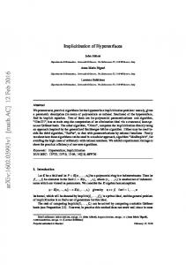
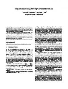
1 Introduction Self-intersection algorithms are important for many applications within CAD/ CAM. Suppose we try to create an offset surface within a CAD system with an offset distance larger than the radius of curvature at some points on the surface. Offset surfaces are not in general rational, and it is therefore necessary to make a NURBS approximation. In a typical CAD-system, surfaces are often represented in terms of degree (3, 3) NURBS surfaces. A NURBS approximation of such an offset surface is shown in fig. 1. We would like to have parts of this surface trimmed away, or maybe even to have it rejected as an illegal surface. This requires an algorithm to find the self-intersection curves, or at least to detect that there are self-intersections. Implicitization is the process of converting a parametric representation of a curve or surface into an implicit one. Figure 2 shows the implicit representation of a cubic curve with a node, given by the zero contour of the implicit function. Implicit representations have many uses. One example is finding intersections between different objects. Ray tracing is a simple case of this, where the parametric form of the ray – a straight line – is inserted into the implicit equation for a surface in order to get an equation in the parameter of the ray. This can then be solved to find the point, or points, of intersection. Note that self-intersections cannot be treated in this relatively simple way because inserting the parametric form into the implicit form for the same object gives identically zero. Thus, finding true self-intersections is a much harder problem. ?
This work was supported by the EU project GAIA II, IST-2001-35512
156
J.B. Thomassen
Fig. 1. NURBS approximation of an offset surface. Made within the CAD-system ’thinkdesign’ from CAD-vendor think3.
0.04 0.02 0 -0.02 -0.04 -0.06 -0.08 3 2 -10
1 -8
-6
-4
0 -2
0
2
-1 4
6
8
-2 10 -3
Fig. 2. Implicit representation of a nodal cubic
In this paper, we discuss an algorithm for finding self-intersections of NURBS curves and surfaces. This algorithm has in part grown out of the long-time experience collected at SINTEF [4, 12], and is still under development. The intersection problem has been studied a lot during the last few decades; for a partial list of references, see [12]. The present algorithm is optimized towards giving certifiable answers with respect to the self-intersections, rather than for speed. Therefore, central to the algorithm is an implicitization step and the use of implicit functions in detecting the self-intersections.
Self-Intersection Problems
157
This will give us more information about the situation and secures the quality of the results compared to many brute force algorithms. Tangential (self-)intersections are in general difficult and will not be considered in this paper. We will therefore assume that all intersections are transversal. Implicitization in CAGD has for a long time meant using classical algebraic techniques like resultants [10, 8] or Gro¨ bner bases [3]. However, it is desirable to use approximate implicit representations of low algebraic degrees, which requires new methods. One recent method is the scattered data fitting method developed by J u¨ ttler et al. [13]. This is very flexible but not accurate or fast. The method of choice for our algorithm is the one developed by Dokken [5, 6], which performs better on accuracy and speed [14]. This method essentially transforms the implicitization problem into the language of linear algebra. As far as we know, this is the simplest way to formulate the problem. In the following, planar B´ezier curves p(t) of degree n are defined in terms of n + 1 control points ci by p(t) =
n X
ci Bi,n (t),
i=0
t ∈ [0, 1],
where the basis functions Bi,n are Bernstein polynomials: µ ¶ n Bi,n (t) = (1 − t)n−i ti . i
(1)
(2)
The unnormalized normal n is defined by n(t) = Rπ/2
dp (t), dt
(3)
³ ´ where Rπ/2 = 10 −1 is a matrix that rotates a vector by an angle of π2 . Implicit 0 curves of degree d are defined in terms of a polynomial function q(x). In the actual implementation of the algorithm we use barycentric coordinates x = (u, v, w) with respect to a triangle enclosing the curve. This improves numerical stability. Thus, for the implicit function we have X q(x) = bijk Bijk,d (x), u + v + w = 1, (4) i+j+k=d
where Bijk,d (x) =
d! i j k uv w , i!j!k!
i + j + k = d,
(5)
are the Bernstein polynomials over this triangle. These 21 (d + 1)(d + 2) monomials constitute a basis for the polynomials of degree d. In barycentric coordinates q is a homogeneous polynomial. We may now sketch the self-intersection algorithm for curves. We are given a NURBS curve of degree n in the plane and we want to find the parameter values that
158
J.B. Thomassen
correspond to self-intersections. Let us assume for simplicity that we are dealing with a non-rational3 parametric curve – that is, the NURBS is in fact a B-spline. 1. Split the curve into B´ezier segments. 2. For each segment p, find candidates to self-intersection parameters. To do this, – find an implicit representation q, – form the quantity ∇q(p(t)) · n(t) and find the roots. 3. For each pair of segments p1 and p2 , find candidates to parameters for ordinary intersections. To do this, – find the implicit representations q1 and q2 , – form the quantities q1 (p2 (t)) and q2 (p1 (t)) and find the roots. 4. Identify parameters for true self-intersections from the list of candidates. To do this, find pairs of parameters from this list whose corresponding 2D points match. Although we have omitted the details, the structure of this algorithm should be straightforward. However, two things we will discuss further is the implicitization and the use of the quantity ∇q(p(t)) · n(t). Thus, in the next section we will discuss exact implicitization. We will show that this is a linear algebra problem – in particular, it is an SVD problem. In sect. 3 we explain why ∇q(p(t)) · n(t) is useful for finding self-intersections. In sect. 4 we start considering surfaces, in particular tensor product B-splines. Unlike for curves, exact implicitization will typically require too high degrees, so if we want an algorithm similar to the one for curves, we need to find an approximate implicit representation. Approximate implicitization is the subject of sect. 5. Finally, in sect. 6 we discuss what are probably the two most important problems to solve before we can get an industrial strength surface intersection algorithm: What degree to choose for the approximate implicitization, and how to find self-intersection curves, as opposed to just points.
2 Implicitization We are given a B´ezier curve p(t) of degree n. We want to find a polynomial q(x) such that the zero-set {x|q(x) = 0} contains p. First of all, we want the degree d of q to be as small as possible for achieving exact implicitization. If p is sufficiently general, then d = n. If the true degree of p is smaller than n, for example if p is obtained by degree elevating a curve of lower degree, we still get an exact implicit representation, but with possible additional branches. This will typically produce phantom candidates for self-intersections in our algorithm, but that is not a problem because of the processing of the candidates at the end of the algorithm. Thus we choose d = n, and we must find a nontrivial 21 (d + 1)(d + 2)-dimensional vector b of coefficients of q such that q(p(t)) = 0. 3
(6)
In this paper, ’non-rational’ means ’polynomial’. This is standard terminology in CAGD, see e.g. Farin’s book [7].
Self-Intersection Problems
159
This turns out to give a matrix equation in b [5, 6]. To see this we calculate q(p(t)) by using the product rule for Bernstein basis functions: ³ ´³ ´ m i
Bi,m (t)Bj,n (t) = ³
n j
m+n i+j
´ Bi+j,m+n (t).
(7)
From this we have that q(p(t)) can be expressed in a Bernstein basis of degree nd. We organize the basis functions in an (nd+1)-dimensional vector B(t) T = (B0,nd (t), . . . , Bnd,nd (t)). Thus we find that inserting p in q yields the factorization q(p(t)) = B(t)T Db,
(8)
where D is an M × N matrix with M = nd + 1 and N = a basis, we see that the problem we need to solve is the matrix equation
1 2 (d + 1)(d + 2).
Since B is (9)
Db = 0.
The standard method for solving a matrix equation like (9) is to use SVD [9]. The theory of the SVD states that we can find the decomposition D = UWV T , where U is an M × N column-orthogonal, W an N × N diagonal, and V an N × N orthogonal matrix. The singular values of D are the numbers on the diagonal of W. The solution to Db = 0 is an eigenvector corresponding to the vanishing singular values in W. If there is exactly one singular value equal to zero, we can find the associated eigenvector from the corresponding column in V. If there are more than one, any linear combination of the corresponding columns will solve (9). Note that we avoid problems with the trivial solution b = 0 to (9). We may always normalize b and thereby q(x). An example of this method of implicitization is the nodal cubic B´ezier curve in fig. 3. The result we have already seen in fig. 2. This implicitization is numerically very exact, and a plot of q(p(t)) as a function of t would show zero to within machine precision. Rational B´ezier curves can be treated in essentially the same way. In barycentric coordinates a rational B´ezier curve is given by Pn wi ci Bi,n (t) p(t) = Pi=0 , (10) n i=0 wi Bi,n (t)
where ci are the control points and wi are the weights. SincePthe implicit function q is homogeneous in barycentric coordinates, the denominator i wi Bi,n (t) leads to a polynomial that factors out in the expression for q(p(t)). PThis means that the nonrational procedure can be applied with just the numerator i wi ci Bi,n (t) instead of p itself.
3 Finding Self-Intersections The other issue we need to discuss is how to find the self-intersections of a B´ezier curve p(t) once an implicit representation q(x) is provided. For each self-intersection point we want to find the two corresponding parameters t1 and t2 such that p(t1 ) = p(t2 ),
t1 6= t2 .
(11)
160
J.B. Thomassen 4
3
2
1
0
-1
-2
-3
-4 -10
-5
0
5
10
Fig. 3. Nodal cubic B´ezier curve
This does not include cusps, which are “degenerate” self-intersections. We will briefly mention cusps later. At a self-intersection point p0 = p(t1 ) = p(t2 ) in the plane the gradient of the implicit function q vanishes: ∇q(p0 ) = 0. In fact p0 is a saddle point of q, which looks like a hyperbolic paraboloid locally around p0 . One way to find the self-intersection parameter values is to form [∇q(p(t))]2 and find the roots of this expression. However, this is not the optimal quantity for this purpose, because the polynomial degree is 2n(d− 1), which is unnecessarily high, and all roots are located at minima. A better choice is the quantity ∇q(p(t)) · n(t),
(12)
where n is the normal. The polynomial degree of (12) is nd − 1. This quantity is proportional to the projection of ∇q on the normal vector along the curve, and has the advantage that it changes sign at roots corresponding to transverse – i.e. non-tangential – self-intersections. For the nodal cubic of fig. 3, the gradient dotted with the normal is plotted in fig. 4. The two roots occur at t1 = 0.25 and t2 = 0.75, which are the correct parameters for the self-intersection. Roots of ∇q · n should be regarded as candidates for self-intersections. Indeed, ∇q may vanish along the curve p(t) if q is reducible so that the additional factors represent extra branches, or if p(t) reaches the endpoint, as we increase t, before the curve has time to complete the loop and self-intersect. This is why the last step of the algorithm is needed.
Self-Intersection Problems
161
0.0004
0.0003
0.0002
1e-04
0
-0.0001
-0.0002
-0.0003
-0.0004
0
0.2
0.4
0.6
0.8
1
Fig. 4. ∇q · n for the nodal cubic of fig. 3
4 Surfaces We now turn to surfaces. In this case we are given a tensor product NURBS surface. Let us assume this to be non-rational. Thus the surface consists of tensor product B´ezier patches: X cij Bi,n1 (u)Bj,n2 (v), (13) p(u, v) = i,j
where the degree is (n1 , n2 ) and cij are the (n1 + 1)(n2 + 1) control points. The unnormalized normal vector n(u, v) is defined by n(u, v) = ∂u p(u, v) × ∂v p(u, v).
(14)
Like for curves we use barycentric coordinates x = (u, v, w, x) in our implementation, this time defined over a tetrahedron enclosing the surface. Then algebraic functions of degree d can be written X q(x) = bijkl Bijkl,d (x), u + v + w + x = 1, (15) i+j+k+l=d
with Bijkl,d (x) =
d! ui v j w k xl , i!j!k!l!
i + j + k + l = d,
(16)
the tetrahedral Bernstein basis. The polynomials Bijkl,d are now the 61 (d+1)(d+2)(d+ 3)-dimensional basis of degree d functions. Again, in barycentric coordinates q(x) is a homogeneous function. What we want now is an algorithm for finding self-intersections like the one for curves. Ideally this would look like:
162
J.B. Thomassen
1. Split the surface into B´ezier patches. 2. For each patch p(u, v), find candidates to self-intersection curves in the (u, v)plane. To do this, – find an implicit representation q, – form ∇q(p(u, v)) · n(u, v) and find the roots. 3. For each pair of patches p1 (u, v) and p2 (u, v), find candidates to parameter curves for ordinary intersections. To do this, – find the implicit representations q1 and q2 , – form q1 (p2 (u, v)) and q2 (p1 (u, v)) and find the zero curves in the (u, v)-plane. 4. Identify the curves in the parameter plane for true self-intersection curves from the list of candidates. To do this, find pairs of parameter curves from this list whose corresponding 3D curves match. Unfortunately it is difficult to implement the algorithm in this way. There are essentially two problems. First, the necessary degree for exact implicitization is too high, both with respect to numerical stability and to speed. Hence the need to find an approximate implicit representation. For a chosen degree, the next section provides a review of how this can be done along the lines of the exact implicitization of sect. 2. However, this leads to the problem of what degree to choose. Second, self-intersection curves are difficult to handle. In the current implementation of the algorithm, we have settled for a compromise to both these problems. We choose d = 4 for the approximate implicitization, based on the expectation that this degree is high enough to capture even complicated topologies. Our experience with this choice is good. Furthermore, instead of working with full self-intersection curves in the parameter plane, we work with points sampled on them. A sampling density must then be chosen, and a density of roughly 100 × 100 in the parameter plane for each patch gives acceptable results. These two compromises lead to a change in the last step of the algorithm, since now also an iteration procedure is required for matching the points in 3D. This matching works roughly as follows. We loop over every pair of points from the list of candidates. Each pair of points in the (u, v)-plane corresponds to two points on the surface. We consider the squared Euclidean distance in 3D space between these two surface points. This is a four-variate function depending on the u and v parameter for the first and second points. Now we look for a minimum of this function. This is where the iterations come in – in our current implementation, a conjugate gradient method is used. If the iteration converges, and if the found minimum is a zero of the distance function, then we have a match and we record the corresponding parameters as points on a selfintersection curve. Then we go on with the next pair, etc. The points found in this way will in general not coincide exactly with the candidates we started with, but they still have the property that they lie on self-intersection curves. An example is given by the offset surface we have already seen in fig. 1. As mentioned in the introduction, this is a realistic industrial example. It consists of many (rational) polynomial surface patches and has a very complex self-intersection structure. The result of running our algorithm on this surface is shown in fig. 5, where we have plotted points in the parameter plane that corresponds to points on the self-intersection curves in 3D space.
Self-Intersection Problems
163
1
0.8
0.6
0.4
0.2
0
0
0.2
0.4
0.6
0.8
1
Fig. 5. Self-intersection points in the parameter plane of the offset surface in fig. 1
5 Approximate Implicitization Although approximate implicitization is mostly relevant for surfaces, we will use curve language for simplicity in the following discussion. However, the results can easily be transferred to the surface case. An implicitly defined curve q(x) = 0 approximates a parametric curve p(t) within the tolerance ² if we can find a vector-valued function ∆p(t) such that q(p(t) + ∆p(t)) = 0
(17)
max |∆p(t)| ≤ ².
(18)
and t
∆p does not need to be continuous. In fact, for nontrivial topologies like self-intersections, p + ∆p may jump from one branch of q to another as we increase t. We may Taylor expand (17) in ∆p around p: q(p(t)) + ∇q(p(t)) · ∆p + · · · = 0.
(19)
Thus, provided ∆p is small and the coefficients of q are normalized in some way, the quantity maxt |q(p(t))| is a meaningful measure of how well q approximates p. This quantity is the “algebraic distance”. How do we find an approximate implicit function q such that the algebraic distance is as small as possible? Again we get an answer from linear algebra. If we insert the B´ezier segment p(t) into a function q with unknown coefficients b we obtain the factorization in eq. (8), q(p(t)) = B(t)T Db.
(20)
164
J.B. Thomassen
Since B(t) is a Bernstein basis, kB(t)k ≤ 1 for all t ∈ [0, 1]. Thus we get the inequality max |q(p(t))| ≤ kDbk. t
(21)
Furthermore, the theory of the SVD tells us that min kDbk = σmin ,
kbk=1
(22)
where σmin is the smallest singular value of D. If we choose the corresponding eigenvector bmin as the coefficients of q we have max |q(p(t))| ≤ σmin . t
(23)
Thus, choosing the vector bmin of coefficients gives us the implicit function we are looking for. If we choose an algebraic degree d for q much lower than the required degree for exact implicitization, it may be that even the smallest singular value σ min is greater than a given tolerance ². It is then possible to improve the situation by subdividing. This leads us to consider convergence rates for approximate implicitization. Let us consider a curve p(t) and pick out an interval [a, b] ⊂ [0, 1] from the parameter domain with length h, that is, b − a = h. If we approximate the curve on this interval by an implicit function q(x) of degree d we will have |q(p(t))| = O(hk+1 ),
t ∈ [a, b],
(24)
as h goes to zero, where the integer k + 1 is the convergence rate. Dokken [5] proved that k = 21 (d + 1)(d + 2) − 2. Likewise for a surface p(u, v) we get a convergence rate from |q(p(u, v))| = O(hk+1 ) (25) ¥ √ ¦ with k = 61 9 + 132d + 72d2 + 12d3 − 23 (see [5]). The notation b· · · c means that ’· · · ’ is rounded downwards to the nearest integer. Thus, for surfaces an approximate implicitization of degree 4 will have convergence rate O(h7 ). If we are not satisfied with the algebraic distance we get from implicitizing a surface, we may dramatically improve the situation with a few subdivisions of the parameter plane. It is therefore a useful strategy to include subdivision in a self-intersection algorithm that is based on implicitization.
6 Two Open Problems Finally, in this section we address the two problems mentioned previously: What degree d should we choose for the implicit representation of a surface in our algorithm? And, also for surfaces, how do we describe and find self-intersection curves, as opposed to just points?
Self-Intersection Problems
165
6.1 What Degree d Should we Choose? For NURBS curves there is no problem with using the required degree for exact implicitization in our algorithm. That is, for a curve of degree n, we may use d = n. For all realistic test cases we have tried, this gives a fast and reliable algorithm. For a NURBS surface of degree (m, n), the required degree for exact implicitization is in general d = 2mn. Thus the realistic case of degree (3, 3) surfaces needs d = 18. A polynomial in 3D of this degree will in general have 1330 terms, which gives very poor precision and long evaluation times. Furthermore, the matrix D in the implicitization becomes so large that the SVD is very slow and has problems with converging. There are several possibilities to overcome this. One is to choose some fixed low degree d and hardcode this in the algorithm. Another is to use some adaptive procedure where we start with a low value for d and then increase it until some requirement is met. We have experimented with both of these possibilities. The requirement in the adaptive procedure was that the smallest singular value in the SVD of D should be smaller than some number. However, it turned out to be very time consuming and not noticeably better than the hardcoding possibility. As already mentioned, d = 4 leads to acceptable results in all test cases we have tried. Could we just as well manage with d = 3, which might lead to a faster algorithm? After all, implicitly defined surfaces of degree 3 are the simplest ones that may exhibit self-intersection curves. However, for d = 3 it turns out that the quality of the candidates to self-intersection points obtained from sampling the zeros of ∇q·n are very poor. This means that the iteration procedure in the matching step leads either to discarding most of the candidates or to produce a large number of redundant matches which is time consuming. On the other hand, for d = 4 iteration leads to matching for most of the candidates without too much redundancy. An example is the surface shown in fig. 6, which has a closed self-intersection curve. The degree of the exact implicit representation is 6. Candidates and the result after iteration for d = 3 is shown in fig. 7, while the result for d = 4 is shown in 8. Nevertheless, it is a suboptimal solution to hardcode the degree once and for all. It would be better to be able to determine for each surface patch which degree would be most suitable. But for the moment it is an open problem how to do that efficiently inside the algorithm. 6.2 How do we Find Self-Intersection Curves (as Opposed to Points)? A possible strategy to finding self-intersection curves is to first find points on these curves and then use a marching technique to “march them out”. The goal here would be to obtain a description of the intersection curves in terms of B-spline (or NURBS) curves in the parameter domain. We have already said a lot about finding such points, so let us discuss marching. Marching is an iterative procedure, which can be used to trace out intersection curves [1, 2] (see [12] for more references). We start with a point on or nearby the curve, and then proceed by taking small steps at a time in a cleverly chosen direction until some stopping criterion is met. For instance, we stop when we reach the edge of the parameter domain or when the curve closes on itself.
166
J.B. Thomassen
Fig. 6. Surface with points on self-intersection curve. Supplied by think3.
1
Candidates Self-intersections
0.8
0.6
0.4
0.2
0
0
0.2
0.4
0.6
0.8
1
Fig. 7. Parameter plane with candidates and self-intersections obtained after iteration for the surface in fig. 6 for Degree 3
One problem we are faced with when marching out a self-intersection curve is the marching onto a singularity, which in this case means a point on the surface where the unnormalized normal vanishes. The normal is used in order to find the direction of the next step in the marching. A singularity of this kind is a cusp. For example, the surface in fig. 6 has two singularities, plotted in fig. 9. Closed self-intersection curves typically have singularities on them.
Self-Intersection Problems 1
167
Candidates Self-intersections
0.8
0.6
0.4
0.2
0
0
0.2
0.4
0.6
0.8
1
Fig. 8. Parameter plane with candidates and self-intersections obtained after iteration for the surface in fig. 6 for Degree 4 1
Self-intersections Singularities
0.8
0.6
0.4
0.2
0
0
0.2
0.4
0.6
0.8
1
Fig. 9. The parameter plane of the surface in fig. 6, with self-intersection points and two cusp-like singularities
Thus, the solution is to identify all the isolated singularities and start the marching from these points. It is not difficult to find isolated cusp singularities. For instance, we may look for the zeros of [n(u, v)]2 , which are also minima. Unfortunately in real life things are not that easy. It may often happen that entire curves of cusp singularities exist. An example of this is the surface in fig. 10. Points sampled from the cusp curves and self-intersection curves in the parameter plane are plotted in fig. 11. As we may see from the plot, in order to start marching we would need
168
J.B. Thomassen
Fig. 10. Bent pipe surface with “supersingularities”. Surface provided by think3.
Self-intersections Singularities
300
250
200
150
100
50
0
0
50
100
150
200
250
300
Fig. 11. Parameter plane of the pipe surface with self-intersection points and points on the cusp curves
to locate an intersection point between a self-intersection curve and a cusp curve. This is a very special kind of singularity, let us call it a “supersingularity”. At the moment we do not know how to properly characterize and find such supersingular points. Until we do, the treatment of self-intersection curves in such cases is another open problem.
Self-Intersection Problems
169
7 Conclusion We have described how we may use implicit representations of curves and surfaces in an algorithm for finding self-intersections. We have also described how to find the implicit representation given a NURBS curve or surface. We do this by formulating it as a linear algebra problem. For curves we may use an exact implicitization, while for surfaces it is necessary to use an approximate implicitization. By using the implicit representation q and the normal vector n we are able to find candidates for the parameters of self-intersections by looking for the roots of ∇q ·n. For curves, where we use exact implicitization, the self-intersection parameters are included in the list of candidates. For surfaces, it is necessary to process the candidates with an iterative procedure to match them in order to get points on the self-intersection curves. Surfaces are much more challenging than curves, and we have described two open problems: How do we choose the degree for the approximate implicitization, and how do we deal with the fact that self-intersections are in general curves? Acknowledgements I thank Tor Dokken for discussions, and for reading and commenting on the manuscript.
References 1. C.L. Bajaj, C.M. Hoffmann, R.E. Lynch, and J.E.H. Hopcroft, Tracing surface intersections, Computer Aided Geometric Design 5 (1988) 285–307. 2. R.E. Barnhill, and S.N. Kersey, A marching method for parametric surface/surface intersection, Computer Aided Geometric Design 7 (1990) 257–280. 3. D. Cox, J. Little, and D. O’Shea, Ideals, Varieties, and Algorithms, Second Edition, SpringerVerlag, New York, 1997. 4. T. Dokken, V. Skytt, and A.-M. Ytrehus, Recursive Subdivision and Iteration in Intersections and Related Problems, in Mathematical Methods in Computer Aided Geometric Design, T. Lyche and L. Schumaker (eds.), Academic Press, 1989, 207–214. 5. T. Dokken, Aspects of Intersection Algorithms and Applications, Ph.D. thesis, University of Oslo, July 1997. 6. T. Dokken, and J.B. Thomassen, Overview of Approximate Implicitization, in Topics in Algebraic Geometry and Geometric Modeling, AMS Cont. Math. 334 (2003), 169–184. 7. G. Farin, Curves and surfaces for CAGD: A practical guide, Fourth Edition, Academic Press, 1997. 8. R.N. Goldman, T.W. Sederberg, and D.C. Anderson, Vector elimination: A technique for the implicitization, inversion, and intersection of planar rational polynomial curves, Computer Aided Geometric Design 1 (1984) 327–356. 9. W.H. Press, S.A. Teukolsky, W.T. Vetterling, and B.P. Flannery, Numerical Recipes in C, Second Edition, Cambridge University Press, 1992. 10. T.W. Sederberg, D.C. Anderson, and R.N. Goldman, Implicit Representation of Parametric Curves and Surfaces, Comp. Vision, Graphics, and Image Processing 28, 72–84 (1984). 11. T.W. Sederberg, J. Zheng, K. Klimaszewski, and T. Dokken, Approximate Implicitization Using Monoid Curves and Surfaces, Graph. Models and Image Proc. 61, 177–198 (1999). 12. V. Skytt, Challenges in surface-surface intersections, these proceedings.
170
J.B. Thomassen
13. E. Wurm, and B. J¨uttler, Approximate implicitization via curve fitting, in L. Kobbelt, P. Schr¨oder, H. Hoppe (eds.), Symposium on Geometry Processing, Eurographics, ACM Siggraph, New York 2003, 240–247. 14. E. Wurm, and J.B. Thomassen, Deliverable 3.2.1 – Benchmarking of the different methods for approximate implicitization, Internal report in the GAIA II project, October 2003.