Executable Specifications with Data-flow Diagrams - Semantic Scholar

SOFTWARE—PRACTICE AND EXPERIENCE, VOL. 23(6), 629–653 (JUNE 1993)

Executable Specifications with Data-flow Diagrams alfonso fuggetta

CEFRIEL, Via Emanueli 15, 20126 Milano, Italy, and Dipartimento di Elettronica e Informazione—Politecnico di Milano, Piazza Leonardo da Vinci, 32, 20133 Milano, Italy

and carlo ghezzi, dino mandrioli and angelo morzenti

Dipartimento di Elettronica e Informazione—Politecnico di Milano, Piazza Leonardo da Vinci, 32, 20133 Milano, Italy

SUMMARY Specifications of information systems applications are often based on the use of entity–relationship (ER) and data-flow diagrams (DFD), which cover, respectively, the conceptual modelling of data and funtions. This paper introduces VLP: an executable visual language for formal specifications and prototyping which integrates ER and DFD diagrams in a semantically rigorous and clear way. Unlike existing commercial products (so-called CASE tools), which can support goodquality documentation, simple forms of consistency checking and bookkeeping, VLP also supports executable specifications, which provide a prototype of the desired application. After reviewing the principles of VLP, the paper outlines the structure of the ECASET environment in which VLP is embedded. In particular, it shows how the environment supports the stepwise derivation of specifications, from informal to formal, and how it supports specification-in-the-large. key words: (Formal) specifications Information systems diagrams Interpretation Prototyping

CASE tools Entity–relationship diagrams Dataflow

INTRODUCTION System analysis and specification are essential activities in any system-development model. Their purpose and objectives are discussed in much detail, often with different perspectives, in most software engineering textbooks (e.g. References 1–3). The nature of this activity is essentially exploratory: the designer examines the application from different viewpoints and at different levels of abstraction, in order to be able to produce the final specification document. This document plays a dual role. On the one hand, it may become part of the contract between the designer and the user; on the other, it is the reference document and the starting point for the development of the application. The languages used to describe specifications cover a broad range: from informal to formal, from those oriented towards embedded, real-time applications, to those oriented towards conventional DP-type applications and information systems. In most 0038–0644/93/060629–25$17.50  1993 by John Wiley & Sons, Ltd.

Received 14 April 1989 Revised 16 November 1990

630

a. fuggetta et al.

practical cases, specifications are written informally, using narrative text; typically, they can include tables, diagrams, and other graphical notations which can convey information in a concise, rigorous, and readable way. Very often, specifications cover two complementary aspects: the data to be handled and the functions that access and manipulate the data. This is especially (but not exclusively) true for applications of information-system type. In this case, it is common to start with the conceptual model of data, often given by entity–relationship diagrams (ERDs).4 Then functionalities are described by means of data-flow diagrams (DFDs). References 5 and 6 illustrate two variations of a popular method to perform analysis and specify functional requirements via DFDs, called structured analysis. Both ERDs and DFDs are graphical notations which communicate requirements in a highly expressive and easy-to-understand way. This is why they have become extremely popular among practitioners, and hence why numerous toolsets exist on the market at present that support specifications using DFDs and ERDs (for example, see Reference 7). Such toolsets fall into the category of CASE (computer aided software engineering) tools. Even though present CASE tools display a wide variety of functionalities, they all share a common weak point: the lack of rigorous semantics of the underlying model. For example, the semantics of DFDs and the relationship between DFDs and ERDs are not formally specified; the interpretation of these and other ambiguous or vague aspects is hidden within unstated assumptions made by the user of the notation. The main consequence of this lack of rigour is that specifications cannot be analysed formally for consistency or correctness, apart from some minor (mostly syntactic) aspects. In particular, specifications usually cannot be executed, and it is not possible to generate code automatically starting from specifications: today’s available CASE tools can at most generate only a small portion of code for some programming languages, such as COBOL (typically, form definitions and code skeletons), or Ada. Nevertheless executability is an attractive property of specifications. 8 An executable specification can be viewed as a prototype of the application being developed; thus it can be used to assess the adequacy of the requirements and give early feedback from the users to software designers before a lengthy and costly development takes place. The potential advantages of prototyping have been widely recognized in the literature,9–11 although its usage is far from being common practice in the development of applications. The basic reason for this is the lack of appropriate tools supporting prototyping. Most of the so-called prototyping aids advertised in the marketplace are just toolsets centred around some high-level language and a database management system. Such toolsets can shorten the development time with respect to traditional approaches. However, they usually do not provide any support to derive intermediate products that can be used in an exploratory fashion to refine requirements in cooperation with the user. Our viewpoint is that the prototype should be a natural offspring of the specification activity; ideally, it should not require an ad hoc development process. A similar viewpoint has been advocated by Kemmerer.12 In order to match our goal, a support environment for specifications should satisfy the following requirements: 1. The environment should be highly interactive and flexible in order to support the exploratory attitude that characterizes specifications.

executable specifications

631

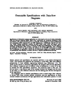
2. Specifiers should be allowed to submit specifications incrementally, with smooth progression from informal to formal. 3. The specification language should be graphical and based on well-known notations that have proved to be widely applicable in the application domain (in our case, applications of information-system type). 4. Specifications should be processable automatically: they should be checkable and executable. The above requirements are exactly the ones we have assumed in our project. According to requirement 4, the specification language must be based on a formal model. However, even if the underlying specification language is formal, the specifier should be allowed to leave parts of the specification undetailed, incomplete, and possibly even inconsistent if he or she so desires. The system should prompt the specifier about possible incompleteness and inconsistencies, but it should be able to tolerate them as long as the designer consciously decides to tolerate them. For example, the designer might decide to work out the details of some parts of the system which deserve a formal treatment, whereas specification of less critical parts might be left at an informal stage. As a consequence of these requirements, the system should be able to adapt the depth and accuracy of its capability of mechanical elaboration to the degree of formality of specifications. As we shall see, this means that the amount of checking and the effectiveness of execution can vary according to the level of formality. The next two sections of the paper describe the formal model underlying VLP, the visual language we have designed for writing specifications. Specifically, the first of the sections develops a formal model for the data-flow component of VLP; the second describes its integration with the entity–relationship component. The two sections following that discuss the overall structure of the ECASET environment which supports VLP specifications, and some implementation issues and the status of the project, respectively. MAKING DATAFLOW DIAGRAMS FORMAL DFDs are one of the most widespread formalisms for requirement specification for data-processing problems, and a variety of software-development methodologies and tools having DFDs as their underlying model7,13 is in use. The popularity of DFDs is largely due to the simplicity and intuitive appeal of their graphical notation: bubbles are used to represent functions resulting from system decomposition, arcs connecting them represent functional dependencies among their input and output data, and suitable visual conventions are provided to represent permanent data stores and data exchange with the external environment. Unfortunately, when used in the specification of complex information systems, DFDs soon reveal their inability to express some kinds of procedural information, since the links between the bubbles represent functional data dependencies, but do not provide all the information regarding control-flow or synchronization conditions that is necessary when specifications are executed. Indeed, the purpose of DFDs is to represent data flow, not control flow; thus specifications given via DFDs are inherently ambiguous and incomplete if we try to interpret them procedurally. The diagram shown in Figure 1, inspired by a similar example of Pressman,3 gives supporting evidence to this argument. The diagram shows the specification of a

632

a. fuggetta et al.

Figure 1. A DFD for a patient-monitoring system

patient monitoring system. The patient’s vital signs (e.g. temperature, blood pressure, ...) are periodically measured and converted to a processable form; they are compared to the patient’s admissible bounds (read from a permanent file), formatted and stored in a data log. If the patient’s data are outside the specified bounds, a warning message is generated for the attention of the nursing personnel. Finally, the nurse can occasionally (i.e. asynchronously) request a report on the patient’s condition: the report is then extracted from the patient’s data log. Apparently, the diagram seems to provide a clear and unambiguous description. However, an attempt to use it to run a simulation of the modelled system would raise some questions that one could answer only by making additional assumptions that could not be based exclusively on the diagram’s composition. For example, one might wonder whether the two activities of ‘patient monitoring’ and ‘patient signs control’ are synchronized in some way and, in particular, whether new data are produced by ‘patient monitoring’ upon request by ‘patient signs control’ when the previously-collected ones have been formatted and stored in the log, or else ‘patient signs control’ is activated when ‘patient monitoring’ produced new data, which might happen at fixed intervals or when significantly different values are measured on the patient. Furthermore, do ‘extract report’ and ‘patient signs control’ interfere with each other’s activity as a consequence of the fact that their respective outputs are directed to the same nurse ‘instance’? Let us consider (for two simpler and more abstract examples) the reasons why DFDs do not provide an adequate notation for specifying control and synchronization between functions. Figure 2 shows a very elementary example, composed of two

Figure 2. A simple DFD


633

connected functions A and B. A’s output is directed as input to B (where the two functions might be part of a larger diagram containing other functions to which both A and B are connected with input and output links. In principle, A and B are two distinct activities, running independently and asynchronously, so a need arises to specify precisely the way in which they interact. In fact, there are at least three different and equally possible ways in which A and B may exchange data. 1. A may ‘produce’ a datum and wait until B ‘consumes’ it before producing another datum, and symmetrically B, after consuming A’s output, may wait until A produces a new one; this would model the situation of a producer/consumer pair, connected via a single element buffer. 2. B may use A’s output more than once, without consuming it, until A will produce (in an asynchronous way) another datum. This may happen in cases where B has other input data, and the datum produced by A is used as a readonly parameter. 3. A and B may have different speeds in producing and consuming data, but a mechanism may be provided for preventing loss or duplication of data (e.g. some kind of finite-length queuing buffer or unbounded pipe). In any case, none of these possibilities is specified explicitly in the diagram of Figure 2, and DFDs do not provide any means to specify any of the above-cited possibilities explicitly. Another typical example of ambiguity of DFD specifications is reported in Figure 3, where three functions A, B, and C are connected as input to D, which sends its outputs to functions E and F. Apart from the above-mentioned synchronization aspects, the diagram does not specify the exact use of D’s input and output data. Again, there are several possibilities; we limit ourselves to citing the following. As far as inputs are concerned, D may need (in order to be activated), all of the data coming from A, B and C, or else D may need only one of A’s, B’s or C’s outputs, and its activation may take place when any one of the three is present, or, finally, D’s activation may depend on more complex combinations of input. For what concerns the outputs, D may give a distinct datum to each of E and F, or it may give the same datum to both E and F, or give the result to either E or F, or we might have more complex cases, such as alternate output to E and F. One might argue that the fuzziness and incompleteness of data-flow diagrams is intentional, since they are often used in phases of the software-development process where procedural details are not relevant and the stress is put exclusively on logical

Figure 3. A DFD ambiguous with respect to the use of function inputs and outputs

634

a. fuggetta et al.

decompositon of the system into modules and on data dependencies. However, sooner or later, more precision is needed, and the notation should allow one to fill in the gap. Moreover, the ambiguity in procedural interpretation and the lack of formality in DFDs prevent their effective use in verification and validation of software, and most important, make it impossible to write executable specifications or to define prototyping tools based on this formalism. In the next two sections we propose a simple model for DFDs, called formal data-flow diagrams (FDFD), which has a precise and unambiguous semantics. To make DFDs formal, one has to give precise rules for synchronization and control in function activation (this will be done in the next subsection) and a formal notation for the definition of the functions and of the data exchanged between them (defined in the subsection after that). To this purpose one might formulate extensions of DFDs that combine them with other specification formalisms to define functions formally, e.g. via decision tables or predicate logic, and to provide a formal execution model (e.g. via Petri nets as in Reference 14, state-transition systems, or finitestate automata). Several such extensions would succeed in making DFDs formal and executable, at the cost of complicating the basic model by introducing extraneous features, thus sacrificing its simplicity and uniformity. Also, extensions to DFDs based on the use of informal notations such as structured English do not address the problems we have raised in the previous sections, since the resulting specifications would not be executable. Instead, we define a simple kernel with a precise and complete semantics, in such a way that any possible new feature (e.g. ‘data repository’ or the ‘signal’ concepts, or any other extension proposed in the literature such as Reference 15) can be defined easily as suitable abstractions built on the basis of the kernel model. FDFDs are the formal model on which VLP is based. Formal data-flow diagrams: synchronization and control To represent synchronization and control conditions explicitly in data-flow diagrams, we propose a model (see also Reference 16) where data exchanged between functions are represented systematically by boxes, as shown in Figure 4, thus eliminating the need for the data sources, sinks and stores of the original DFD model. An FDFD is composed of n data containers (represented by boxes) and m data transformers (represented by bubbles). Each box i is associated with a data type Di, and may contain one value of that type or be empty. A box is connected as input to a bubble when there is an arrow going from the box to the bubble, and is connected as output when there is an arrow in the opposite direction. A data transformer j having k input boxes and p output boxes (see Figure 5) has associated with it a p-valued function fj of the type fj : Dji1 × Dji2 × ... × Djik → Djoˆ1 × Djoˆ2 × ... × Djoˆp

Figure 4. Data container (box) and data transformers (bubbles)


635

Figure 5. A function and its input and output data containers

where Dˆi = Di < {‘null’}:in other words, the function fj may yield, besides values of the types associated with the output boxes, the special ‘null’ value. As we shall show shortly, the ‘null’ value is needed to describe data transformer activation on particular input values. For the moment we do not make any assumption about the ways functions and data types are defined: we shall just assume that there is a suitable formalism to do that, and postpone its discussion to a later section. There are two kinds of connection between boxes and bubbles, which are represented graphically as simple arrows ‘→’ and double arrows ‘→ →’. A simple arrow indicates destructive operations: reading the datum from an input box leaves the box empty, whereas for an output box the newly-computed value cancels the old value that was (possibly) there before data transformer activation. A double arrow row indicates non-destructive operations: for an input box a conservative reading is performed, which does not cancel the previously-present datum, whereas for an output box writing is blocking, which means that the data transformer is not activated unless the box is empty (i.e. the old value has been ‘consumed’ by another data transformer having that box as a non-conservative input). We can now state precisely the conditions under which a data transformer is enabled for execution and the effect of its activation (more formal definitions can be found in Reference 17, where the semantics of this basically asynchronous model is given in terms of a simpler underlying synchronous model). A data transformer is enabled for activation if and only if (a) all input boxes are full, and (b) all blocking output boxes are empty. The activation of the function associated with a data transformer has the following effect on its input and output boxes: (i) all non-conservative input boxes are emptied (conservative inputs remain unchanged), and (ii) all output boxes receive the value newly computed by the function, if this value is not equal to ‘null’; otherwise the contents of the boxes remain unchanged. Note that for a given diagram configuration (that is, combination of box contents), more than one data transformer may be enabled. In this case one of the enabled bubbles is chosen non-deterministically for execution, and the associated function is activated. Thus, the parallel execution of data transformers that are enabled simultaneously is modelled by the sequential interleaving of their executions. Using FDFDs, the different possibilities described for Figure 2 can be specified

636

a. fuggetta et al.

unambiguously. For instance, Figure 6(a) shows functions A and B being connected by a unit-length buffer, and Figure 6(b) a connection via a pipe mechanism. In this Figure, data containers Din and Dout represent input and output buffers to the pipe, where items from A and for B are stored before (after) being enqueued; boxes Din and Dout are assumed to be of type ‘item’. Input connections to these containers are conservative, in order to avoid loss of data. The data container FIFO contains the data sequence that constitutes the pipe; hence its type is ‘sequence of item’. For instance, if the ‘producer’ process A and the ‘consumer’ process B are exchanging a sequence of characters, then the type of data container Din and Dout would be ‘character’, whereas the type of box FIFO would be ‘string’. Initially, the data container FIFO is empty, so that only the data transformer Init can be activated, producing the initial sequence of length zero. From this point on, Init will never be activated, since the data container FIFO is always full, being both input and ouput of ServerA and ServerB. Server A is activated when Din contains a datum to be appended to the pipe, and produces a new pipe that includes the datum from Din. ServerB works in a similar way; notice, however, that when the data container Dout is empty and FIFO contains the sequence of length zero representing an empty pipe, ServerB returns, if activated, a ‘null’ value, thus leaving data container Dout empty. The case discussed in connection with Figure 3 can be modelled in a similar way. A few comments on the above-defined FDFD formalism, and comparisons with similar proposals that have been presented in the literature, are now in order. As stated in the introduction, our main purpose in defining this extension of data-flow diagrams is to provide notations to express control and synchronization information, in order to give them a formal operational semantics as the basis for execution and rapid prototyping tools. Thus, starting from a descriptive formalism like DFD, we have obtained a notation which is more operational in nature, since an FDFD is in fact a complex state machine. Being both asynchronous and non-deterministic, FDFDs are also related to Petri nets; the relationship becomes evident if one thinks of data containers as ‘places’ and of bubbles as ‘transitions’ of the net. Note, however, that a few significant differences between the two models exist; we do not discuss this question in depth, but just mention the fact that at most one single datum may be present at any time in a data container (whereas a place in a Petri net might hold

Figure 6. Unambiguous specification of synchronization among functions


637

any number of tokens) and that conservative connections, especially those for output, have no counterpart in Petri nets. We refer here to the most widely-used version of the Petri net model, as defined by Peterson.18 The subclass known as the condition– event system19 is actually closer to our model. Several other approaches to making DFDs executable have been taken, the common starting-point being the flaws and inaccuracies that were pointed out at the beginning of this section. In Reference 20 a tool for the execution of DFDs is presented, where the DFD formalism is not modified or extended to allow the specifier to add the required information, but rather the ‘DFD interpreter’ interacts with the user in case the execution might proceed in more than one way. Thus the approach seems appealing from an intuitive point of view, and is simple to implement. However, many risks of ambiguity are not avoided, since the same notation can be interpreted in different ways depending on which user is interacting with the system. The approach of Ward15 extends the DFD notation to represent control and timing, by the definition of the so-called ‘transformation schema’. The criterion followed in the extension is the separation of data elaboration from the handling of control, which is pursued by defining explicit signals for the activation and deactivation of data transformations and by introducing control bubbles, whose logic can be specified via finite state automata. However, this separation of control and data processing seems to reflect the typical architecture on which the systems being modelled (industrial-plant control in this instance) are usually implemented, rather than being motivated by reasons of simplicity and modularity. Furthermore, this separation is not thoroughly respected, since data-transforming bubbles can emit signals to control bubbles, in order to indicate that they are done with the processing, and signals may even be emitted by an arbitrary output arc when a datum is present on it. These and other exceptions to the separation of data processing and control make the execution rules for transformation schemas quite intricate and difficult to grasp, also because they are not given in a formal way, but described in (rather informal) English prose. We believe, instead, that data processing and control are often tightly connected, especially in conventional information systems, where the plain presence of a computed or input data value has a clear control meaning. As a consequence, we use data containers to give an explicit representation of data. This choice yields a notation that is simple and elementary but at the same time has a great expressive power and formal and intuitive semantics. The reader may object that very often a purely data-flow-oriented view of the specified system can be useful, especially in the initial stages of specification when control aspects are ignored deliberately. We agree fully with this point, but it can be taken into account by stating suitable requirements for the tool that supports FDFD specifications (see the section on the specification environment, below). For example, the tool might be able to provide a view of the system that would ignore data containers and would output a purely conventional DFD, should the user of the tool request it. Two more comments can be made on the approach adopted by Ward15 in his transformation schemas. First, Ward’s notation is not completely formalized, so that it is not possible to interpret, symbolically execute and test a specification unless further information is provided by the specifier. Secondly, by using the elementary constructs of FDFD, one can easily obtain the more elaborate control structures that he defines: in fact, one of the possible targets of our research is to provide the user

638

a. fuggetta et al.

with ways to tailor his own specification environment by defining new higher level constructs as macros built in terms of the basic features of the FDFD model (see, for example, the pipe defined in Figure 6). The work of Docker and Tate21 shares most of our motivations, and proposes an approach that has significant commonalities with FDFDs: the notation is completely formalized with the purpose of supporting automatic execution of specifications. The execution model is based on the data-flow machine architecture as described in References 22 and 23: each bubble of the DFD represents an asynchronous process that is activated whenever all of its input data are available, and produces one datum for each of its output arcs. A connection between two bubbles corresponds to a pipe of data exchanged by the associated processes. However, FDFDs provide a more general approach, since they make it possible to build pipes starting from the basic objects provided; moreover, both synchronous and asynchronous interactions among processes can be specified using conservative and non-conservative connections. Notice that, in the original formulation of De Marco,5 DFDs are used to provide a rather informal description of several interaction mechanisms among processes. Actually, a variety of inter-process interactions mechanisms is needed in practice to cope with the complexity of real applications; thus, in our opinion, any notation aiming at formalizing DFDs should provide a sufficient degree of flexibility. Formal data-flow diagrams: data and function definition The VLP language is based on the FDFD model where it deals with data transformation; it also includes a formal notation for the definition of the types of data contained in the boxes and of the functions associated with bubbles of the diagrams. Being formal, the notation is executable: it is actually a very-high-level language suitable for rapid prototyping. We shall now briefly review the constructs for the definition of the simpler types of data structures, and for the definition of functions. In the next section we shall show in greater detail how the usefulness of this prototyping tool is substantially increased by the use of the entity–relationship model for the description of data, and by its consistent integration with the above defined data-flow model. Data types may be defined in a way similar to what is done in Pascal-like languages, starting from elementary types (boolean, integer and real numbers, characters etc.) and using the usual aggregate constructors, array and record, to which the pipe constructor has been added due to its frequent use in practical applications. The pipe is essentially a short notation for the diagram shown in Figure 6(b). The following declarations define data types which may be of interest in the administration of a chain of hotels. type Client is record FirstName: string [15]; LastName: string [25]; Smoker: boolean; ... end record; type Room is record


639

RoomNo: integer; Name: string [15]; TVSet, View, Smoker: boolean; DailyPrice: integer; ... end record; type Hotel is record Name: string [15]; City: string [20]; Country: string [10]; Category: [1..5]; ... end record; type Party is pipe of Client;

Note: Although the type of a data container is given in a pure textual form, the definition is actually entered by interacting with the graphical editor via dialogue boxes, as we show in the section on the specification environment. Functions are defined in a strongly-typed high-level language. A terminal data transformer (i.e. a data transformer that is not refined in terms of other diagrams, see the section just mentioned) may contain a call to one of these functions. Such functions are external to one another, and their execution does not have any sideeffect: the only way they can modify the state of the diagram is through their parameters. Thus, the header of a function declaration will contain a list of the function’s input and output parameters, according to the following pattern: function kfunction namel (input kformal input parameter listl; output kformal output parameter listl);

Functions will contain a declarative part where local variables may be defined, and an executable part consisting of composition of the usual instructions of structured programming (assignment, conditional and branching instructions, iterative instructions, function calls). No local function declaration is allowed, and no recursion, either direct or indirect, is admitted. INTEGRATING ENTITY–RELATIONSHIP AND DATA-FLOW DIAGRAMS Besides the data constructors presented in the last sections, the VLP language gives the user a set of primitives for the definition of data according to the entity– relationship model,4 and for their graphical representation with conventions completely consistent with those adopted for ordinarily-structured data. To obtain a complete integration between DF and the ER models, the function-definition language is also enriched with operators and instructions for the manipulation of entities and relations. The language provides the above-cited array, record and pipe constructors, plus two new aggregate constructors for the definition of collections and relations. A collection is a set of elements, each element being a record object composed of distinct fields, some of which are specified as key fields. No repetitions are allowed in a collection; that is, all its elements must have different values for their key

640

a. fuggetta et al.

fields. As an example of collection type definitions, let us consider the following, which defines groups of clients, uniquely identified by their first and last names, collections of rooms, identified by a pair room number /identifier, and collections of hotels, identified by the pair name / city. type CollClients is collection of Client key [FirstName, LastName]; type CollRooms is collection of Room key [Name, RoomNo]; type CollHotels is collection of Hotel key [Name, City];

A relation is a set of links between pairs of collection elements, where each pair of links might be attached to some attributes, called the set of attributes of the relation. Relations are thus binary; if further information is logically related to each relation element, this can be added to it as an attribute. Like collections, relations cannot contain duplicates: no two relation elements are allowed to link the same pair of collection elements. A relation may be represented, at a rather intuitive level, as in Figure 7, where we show two collections as sets and a relation existing on them as a set of links between elements of the two collections, with the attributes attached to each relation element. Relations may be partial, that is, not all elements of the collections involved are necessarily connected to a relation element, and may be one-to-one, one-to-many, many-to-one, or many-to-many, with the usual meaning. The definition of a relation is performed in two steps: first, a declaration of the type of the relation must be provided, which specifies the type of the collections involved, the attributes (when present) and the cardinality of the relation; afterwards specific instances of that relation type may be created by an object declaration which cites as an additional constraint the names of the relevant collection objects, which obviously must be of the collection types requested by the relation type declaration. For a practical example, let us return to the hotel chain, where we suppose that every hotel can provide many rooms (which, of course, belong to that unique hotel), any client may reserve one or more rooms in any hotel, and after the client’s departure from any hotel of the chain a record is kept of his/her stay. This situation can be described in terms of our entity–relationship model by means of the following type and object declarations (notice that the symbol ‘?’ is used to represent a ‘many’ cardinality in a relation type declaration):

Figure 7. A concrete representation of a relation among two collections


641

type ClientsHotels is relation [CollClients, CollHotels] cardinality [?:?] with Date;

where Date is the type specified by the following declaration: Date is record Day: [1..31]; Month: string [10]; Year: [1900..2100]; end record; type ClientsRooms is relation [CollClients, CollRooms] cardinality [1:?] with Conditions;

where Conditions is defined as Conditions is record Start, End: Date; ... end record; type HotelRooms is relation [CollHotels, CollRooms] cardinality [1:?]; Clients: CollClients; Rooms: CollRooms; Hotels: CollHotels; Reserved: ClientsRooms [Clients, Rooms]; Stayed: ClientsHotels [Clients, Hotels]; Provides: HotelRooms [Hotels, Rooms];

This amounts to declaring three collections for the Clients, the Rooms and the Hotels, modelling reservations as a one-to-many relation between Clients and Rooms, the stays of the clients as many-to-many relations between Clients and Hotels, and the fact that one hotel has many rooms as a one-to-many relation between Hotels and Rooms. Now, collection and relation objects are represented by the prototyping tool as data containers and treated accordingly: they can be connected, as both conservative and non-conservative input and output, to bubbles. Since collections and relations are represented in the diagrams as data containers, their definition, although given above in a pure textual form, is actually entered by the user when interacting with the graphical editor that is used to construct the diagrams. To distinguish the objects belonging to the entity/relationship model visually, special conventions are adopted for their data containers: collections are represented graphically as double-bordered rectangles, and relations as diamonds. Relation containers are also connected to their collections using dashed lines, to distinguish these connections from those originating from the data-flow part of the diagrams. Adopting a widely-accepted convention, these connections between relations and collections are terminated with the tip of an arrow on the sides where the relation has cardinality one. Keeping all these

642

a. fuggetta et al.

graphical conventions in mind, data regarding hotels, rooms and clients may be represented by the portion of diagram reported in Figure 8. The language provides primitives for the manipulation of collections and relation objects. In particular, the following operations are allowed: (a) adding and deleting an element to and from a collection or a relation* (b) modifying the attributes of a collection or relation element* (c) selecting parts (i.e. subsets) of a collection or a relation, possibly projecting them on some of the attributes. The following constraints must be met when performing any operation on collections and relations, in order to keep the data in a consistent state. 1. Values of key attributes of a collection element cannot be modified: the element must be deleted and another one with different key attributes must be inserted. 2. One cannot delete a collection element that is linked to a relation element: the latter must be deleted first. 3. No duplication of relation and collection elements is allowed. All these constraints on relation and collection operations are checked at run-time by the interpreter of the prototyping environment. The primitives for manipulating collections and relations also make possible the selection of element(s) according to conditions composed using (besides the usual logical operators) existential and universal quantifiers. This results in a very-highlevel language, which reminds one of the notation of first-order theories. Rather than giving a lengthy detailed account of the syntax and semantics of these operators, we shall present a few examples of their application to the data structures defined above for the hotel-chain example; for the sake of simplicity, we keep the same names for all the objects (although, inside functions, the names of the formal parameters, not those of the data containers, would be used). The room with name ‘Belvedere’ and number 256 can be selected with the expression the room in Rooms suchthat (room.Name = “Belvedere” and room.RoomNo = 256)

Figure 8. Data regarding the hotel chain according to the ER model * Notice that these operations do not contradict the functional paradigm adopted in the specification language, since they are not performed through side-effects but (at least conceptually) by producing brand-new objects.


643

and its DailyPrice attribute may be assigned the new value of $250 by the following instruction the room in Rooms suchthat (room.Name = “Belvedere” and room.RoomNo = 256).DailyPrice := 250;

The expression all room.RoomNo, Name, DailyPrice in Rooms suchthat (exist (elem in Provides suchthat (Rooms (elem) = room and Hotels (elem).City = “Florence” and Hotels (elem).Category # 2) and room.View and room.DaileyPrice # 300)

produces as its value a collection composed of the number, name, and prices of rooms with a view, in a second—or better—category hotel of Florence, that cost less than $300. Special instructions are also provided to perform iterative instructions on collections and relation elements, and the operator count determines the number of elements satisfying a specified property. Thus the composite instruction forall client in Clients suchthat (count stay in Stayed suchthat (stay.End.Year$CurrentYear − 1 and Clients(stay) = client ) $ 2) do {send a greeting letter to client}; od;

writes a greeting message to the most faithful clients: those who have stayed at least twice in a hotel belonging to the chain during the previous two years. These examples should give an idea of the primitives offered by VLP for manipulating collections and relations. A complete and precise view of the language is given in the reference manual.24 OUTLINE OF THE SPECIFICATION ENVIRONMENT The VLP specification language has been developed within the context of joint research between industry and university, with the aim of providing an advanced specification environment that will enable the designer to produce and analyse executable specifications.25 This project, called ECASET, has developed a tool which provides the following functionalities: 1. Graphical editing: it allows the designer to lay down a VLP specification through a graphical editor which includes the editing features that can usually be found in commercially-available CASE tools. 2. Interpretation: it allows the designer to switch easily from specification to prototyping, by a direct execution of the VLP specifications.

644

a. fuggetta et al.

The two components (the editor and the interpreter) are not different packages to be activated in sequence: they constitute different functionalities of the same tool. The designer can switch quickly from specification to prototyping and back to specification, by simply selecting different menu items. Moreover, the interpreter is able to manage partially-specified VLP specifications—as we will see in more detail later in the present section—thus allowing the user to see the result of his/her work even in the early stage of the design process. Modules, refinement and atomic execution The specification unit that can be handled by ECASET is called a module: it is composed of a VLP specification and a set of function and type definitions. A VLP specification is composed of a set of data transformers (bubbles), a set of containers (boxes) and a set of connectors that link data transformers to containers. To each data transformer, we can associate a function call—in this case it is called a terminal data transformer—or it can be refined further through a new VLP diagram—in this case it is called a refined data transformer. Notice that the function call associated with a terminal data transformer can correspond to a textually-defined function or to a function defined diagrammatically by means of a separate VLP specification. In the latter case, in order to define a function, a VLP diagram must be state-free; i.e. it must not keep track of previous executions in its internal boxes. It is not possible to assign a function call to a refined data transformer nor to refine a data transformer that already has an associated function call: if this were possible the user could specify two different and possibly inconsistent semantics for the same data transformer. For each refined data transformer, there is an associated VLP specification that defines its semantics in more detail: this description constitutes a level of refinement of the module and must be topologically consistent with the outer level, i.e. it must have the same type of connections with the same containers linked to the corresponding refined data transformer. The level of refinement of a module can be represented by a refinement tree, in which each node is a data transformer, each arc connects a refined data transformer to one of the data transformer in its refinement, and the leaves are terminal data transformers. Each level of refinement is identified by the set of nodes that have the same parent node. With reference to the hotel-chain example, Figures 9 and 10 show a data transformer for room reservation, and the diagram that refines it*. The distinction between terminal and refined data transformers is supported consistently, at run-time, by the interpreter. During execution, the interpreter ignores intermediate levels of the refinement tree: only the leaves of the tree are considered. Thus the interpreter executes only terminal data transformers, by calling their associated functions, and each function-activation is handled as an atomic action. When the function to be activated is defined by a diagram, its activation produces a new level of atomicity. This means that when the interpreter activates a terminal data transformer dt of a VLP diagram D and dt’s associated function is defined by a VLP diagram d, only d’s data transformers can be executed until d is terminated, * In what follows, we shall show several diagrams in which containers that are both input and output of one data transformer are connected by a single double-arrowed connector. Actually, this kind of connector is obtained by drawing two distinct but overlapping connections, and therefore it is not a new VLP construct, but just a graphical notation used to improve readability.


645

Figure 9.

so that execution of the terminal data transformer dt is an atomic action for the caller diagram D. Specification in the large A critical issue in software development is the integration of the activities of different designers working on the same project. Moreover, as software products become bigger and bigger, it is quite complex to manage development teams and processes. At the moment, ECASET provides a limited set of features addressing these problems: its features are based on an integrated project database that stores the description of the ECASET environment. The ECASET environment records information about the users of ECASET and the modules they are developing. Each user has a private user library that contains all the modules he/she has developed so far. A user can access in update mode only modules of his/her library, but can browse (in read-only mode) the modules stored in other users’ libraries. There is a privileged user, called the system administrator, whose library is called the system library: it contains modules that have been released officially by users. The system administrator can perform system-maintenance operations such as creation of new users and system clean-up, and can also access in update mode every module stored in any user’s library. A module can export resources, i.e. function definitions and containers (usually, collections and relations); it can also import resources from other modules of the

646

a. fuggetta et al.

Figure 10.

environment. When a resource is imported by a module, there is no indication of the identity of the corresponding exporting module; similarly, an exporting module does not identify the possible client modules of the exported resource. The binding between imported and exported resources is done when the user requests interpretation of a VLP specification, and is based on the concept of execution environment. An execution environment is a list of the names of modules, belonging to the user’s library or to the system library, that are used to bind import and export resource declarations. In order to be established, a binding is subject to some constraints that we ignore here for simplicity. Editing and executing specifications The functionalities provided by the ECASET editor are based on a graphical user interface which encourages the designer to enter specifications in a very easy way. The editor allows the designer to navigate across a refinement tree via ‘zoom in’ and ‘zoom out’ operations that can be applied to different data transformers. The consistency among different levels of refinement is ensured by the editor: when the designer issues a request, if its processing can produce an inconsistent situation in the refinement tree, the editor does not process the command and warns the user about the illegal operation. Type definitions are entered through dialogue boxes that guide the designer in the


647

definition process. A text editor can be used to associate narrative comments with the objects of a VLP diagram (for example, data transformers or containers). The interpreter is activated via a menu option and performs two operations: (a) it checks the consistency of the execution environment and binds imported to exported resources, and (b) it determines the set of terminal data transformers and then starts the execution. The execution consists of a cyclic evaluation of the set of terminal data transformers that can be activated, and a choice of the data transformer to be activated. A datatransformer activation consists of calling the associated function and modifying the contents of the connected containers, according to results of the function. The interpreter can operate in an automatic mode or be controlled by the user. In the former case it will select the next data transformer to activate according to a policy that is hidden from the user, while in the latter, if it finds more than one data transformer that can be activated, it gives control to the user in order to allow him/her to select the transformer to activate. The user can specify breakpoints: when the interpreter reaches them it suspends the execution of the VLP program and returns control to the user. After suspending execution, the user can request the interpreter to resume its processing. This is possible only if the user has not modified the definition of any object belonging to the execution environment (for example, a connection between a data transformer and a data container, or a function definition); conversely, if edit operations are performed, the values of the local variables are lost and the interpreter must start from scratch. When the interpreter is not active (because the execution is not started yet or is suspended), the user can inspect and modify the contents of containers and of local variables in active functions. One of the main goals of the ECASET project is to provide an environment that allows the designer to detail his/her specifications incrementally: in the early phase of the design, the user may not be able to define a specification completely in a detailed and unambiguous way. Therefore, the designer must be allowed to leave some details unspecified and still be able to test the application, using all information available at that point. Both the editor and the interpreter have been designed in such a way that they can operate also in the case of incomplete information. For example, if during the execution of a specification, the interpreter finds an undefined function, it suspends the execution and requests the user to supply values manually (via the inspect command) for the output parameters, thus simulating the function call. It is also able to manage undefined types via the concept of token. A token is a predefined value that can be stored in any container: a function that is connected to at least one undefined container produces only tokens. This happens also if a defined input container contains a token received by a previously-activated function. Tokens can propagate across the whole diagram: they can be used to have a first rough simulation of the final behaviour of the application under development in terms of pure controlflow. Figures 11, 12 and 13 are examples of how ECASET deals with incomplete specifications. Figure 11 shows the message that ECASET displays on the screen when it encounters an undefined function. Figure 12 shows the initial status of the diagram when the type of data container Request is undefined: placing a token in

648

a. fuggetta et al.

Figure 11.

the container and executing the diagram causes output containers of data transformer Check request to be filled with tokens, and input container Request to be emptied, as shown in Figure 13. It is rather obvious to observe that, in this case, VLP diagrams become even closer to Petri nets, and thus provide similar modelling capabilities. THE IMPLEMENTATION OF ECASET The prototype of ECASET has been developed on MS-DOS-based personal computers using the following tools. 1. Microsoft C compiler 4.026 2. Microsoft Windows Development Toolkit Version 2.0327 3. Informix C-ISAM.28 The target architecture that will host an ECASET-based software-specification environment is a network of personal computers with one machine acting as a server storing the project database and several PCs each running ECASET. The editor provides the user with a set of editing features that facilitate the design activity. Besides typical editing features—such as automatic redrawing of connections when an object is moved, or automatic scrolling of the drawing sheet when the user drags the mouse outside of the window—the editor allows the designer to cut and paste entire refinement subtrees. When the user cuts or copies a refined data transformer, the associated refinement tree is marked: if, at a later moment, a paste


649

Figure 12.

operation is invoked, the system inserts at the current level of refinement a copy of the marked tree, renaming all its VLP objects in order to avoid aliasing. The editor allows the user to display on the screen only the entity–relationship portion of a VLP diagram. As we saw, in VLP it is possible to declare containers of type relation and collection: they are used to implement ER-based data structures. When the editor command ‘ER-only’ is invoked, the editor displays on the screen only containers of type collections and relations, and links (in the ER meaning) among them. A common criterion that has been adopted throughout the project is to give active support to an incremental attitude to the specification activity. As a first example, an ECASET user can create several types of objects: data types, containers, functions. To create them, the user is not forced to follow a predefined path, but can freely take advantage of the ‘forward’ declaration schema of ECASET. Each time the user includes a reference to an undeclared object (e.g. an undeclared type-name), ECASET automatically creates the new object with a set of default values that can be derived by the current set of user’s declarations. At a later moment, the user can complete the declaration, possibly modifying ECASET’s assumptions. During these activities the user is guided by ECASET, which shows him/her only those choices that are compatible with the actual status of the environment. This incremental schema is adopted also to allocate memory space for containers and, as we shall see later, for textual function definitions. As soon as the user completes a new container declaration, ECASET allocates the proper memory space, either in the program-heap area or as new C-ISAM files in order to store data for

650

a. fuggetta et al.

Figure 13.

that container. When the user modifies a container declaration, if the size of the memory needed to store data for that container is changed, ECASET releases the previously-allocated area and repeats the allocation process in order to accommodate the user’s changes. The same approach is adopted in the textual definition of functions. A function defined textually must be compiled in order to produce the code that is actually executed at run-time by the interpreter: thus the compiler is activated each time the user quits the editor confirming his/her updates to the source of the function*. Thanks to the incremental approach sketched above, when the user issues a run command, the amount of work needed for an actual run of the VLP program is greatly reduced since the ‘compiling overhead’ is not concentrated in a single phase: this fact makes it easier for the user to switch quickly from editing to prototyping. As we saw, ECASET is based on a project database (PDB) that stores the information describing the ECASET environment. When the user asks for opening of a module, ECASET loads its description from the PDB and stores it in a set of memory tables that are isomorphic with the PDB files. These tables are primarily used by the editor, since they contain the description of the topology of VLP diagrams, the definition of types and the description of the function headers (name of the function and parameter definitions). All comments and programs (both source and precompiled code) are stored in byte-stream files, whose names are held in the * The compiler has been developed using YACC and LEX and has been embedded in ECASET as a subroutine.


651

PDB (and, therefore, after loading the module, in the main memory tables): when the text editor or the compiler is activated, the selected text is loaded in memory buffers where it is processed. Notice that in the current version of ECASET the entire module is loaded in a statically-allocated region of the main memory and no buffering scheme is provided in order to minimize the amount of memory needed to store this information. This choice has simplified the implementation of the ECASET environment, but prevents the inclusion of features enabling the user to import and export resources across different modules, since it makes it infeasible to load in memory more than one module at a time. This limitation, due to our simplified memory-management scheme, will be removed during the engineering of the product. The compiler generates postfix code for a stack-based virtual machine that has been embedded in the VLP interpreter. This abstract machine provides as primitive operations, among others, instructions for manipulating C-ISAM files. The interpretation process is supported by a run-time stack that is used, as in traditional programming languages, to allocate memory for containers and for local variables of functions. The base of the stack is used to allocate space for containers declared in the main VLP diagram; the contents of the base of the stack are preserved when the module is unloaded from memory and, therefore, can be reused in different sessions of work. A function call is managed, as in traditional programming languages, by creating on top of the stack an activation record that includes (a) memory space for local variables (b) an instruction pointer, describing the point in the caller where the function has been called and the interpreter will eventually return (c) a dynamic link, which is the reference to the stack pointer to the activation record of the calling function. This value will be used to pop the activation record of a terminated function and restore the activation record of the caller function on top of the stack. Pipes, collections and relations are implemented through C-ISAM files, whose identifier is the value actually stored in containers or variables of those types. Both the compiler and the interpreter produce several messages describing their status and the results of their processing. These messages are sent to a special popup window, the ‘system window’, which ECASET opens on top of the drawing sheet: the user can browse through these messages or print them in order to have a written trace of the ECASET activities. CONCLUSIONS AND ACKNOWLEDGEMENTS In this paper we have outlined the ECASET environment and, in particular, we have focused on its kernel: the visual language VLP. A first prototype of the ECASET environment has been developed and is now in service with pilot industrial users. The next step in our research activity will be to investigate new features of the environment to be prototyped. As we have stated early in this paper, we intend to enhance ECASET by introducing a meta-environment that will allow the user to extend VLP by defining new language constructs in terms of the primitive constructs provided by the system. In order to support fully the visual approach adopted in

652

a. fuggetta et al.

VLP, the meta-environment will also allow the user to associate an iconic representation with every user-defined extension. We also plan to address the issues of specification-in-the-large more deeply, and to investigate the problem of automatically deriving test cases from VLP specifications, in order to support functional testing of the resulting implementation.29 Another possible line of investigation will be the problem of translating VLP specifications into a target implementation language and database management system, possibly via program transformations. The deep motivation underlying our work is that the world of data-processingtype applications (which covers the largest majority of today’s applications) may gain advantages from the use of formal specification, provided that software designers can be supported by a flexible highly-interactive environment based on a visual specification formalism. Early practical experience with the ECASET prototype seems to confirm our motivation. acknowledgements The authors wish to thank Roberto Nalbone, for his continuous support, and the members of the ECASET development team, Daria Contardi, Giuliano Locatelli, Marco Malinverni, Fabio Prandelli, Luca Santi and Giovanni Seminati for many helpful comments. Comments provided by the reviewers were also appreciated. This work was funded by ENIDATA and partially supported by CNR-Progetto Finalizzato Sistemi Informatici e Calcolo Parallelo. REFERENCES 1. R. E. Fairley, Software engineering Concepts, McGraw-Hill, 1985. 2. I. Sommerville, Software Engineering, fourth edn, Addison Wesley, Reading, MA, 1992. 3. R. S. Pressman, Software Engineering: a Practitioner’s Approach second edn, McGraw-Hill, New York, 1987. 4. P. P. Chen, ‘The entity-relationship model: towards a unified view of data’, ACM Transactions on Database Systems, 1, 9–36 (1976). 5. T. De Marco, Structured Analysis and System Specification, Yourdon Press, New York, 1978. 6. C. P. Gane and T. Sarson, Structured System Analysis: Tools and Techniques, Prentice-Hall International, Englewood Cliffs, NJ, 1979. 7. S. A. Dart, R. J. Ellison, P. H. Feiler and A.N. Habermann, ‘Software development environments’, IEEE Computer, 20, (11), 18–29 (1987). 8. C. Ghezzi and D. Mandrioli, ‘On eclecticism in specifications. A case-study centred around Petri nets’, 4th IEEE Workshop on Software Design and Specification, Monterey, CA, 1987. 9. B. Boar, Application Prototyping, Wiley, New York, 1984. 10. R. Balzer, T. E. Cheatam and C. Green, ‘Software technology in the 1990’s: using a new paradigm’, IEEE Computer, November 1983, pp. 34–45. 11. R. Balzer, ‘A 15 year perspective on automatic programming’ IEEE Trans. Software Engineering, SE11, (11), pp. 1257–1268 (1985). 12. R. A. Kemmerer, ‘Testing formal specifications to detect design errors’, IEEE Trans. Software Engineering, SE-11, (1), 32–43 (1985). 13. E. Yourdon and L. L. Constantine, Structured Design, Prentice Hall International, Englewood Cliffs, NJ, 1979. 14. T. H. Tse and L. Pong, ‘Towards a formal foundation for DeMarco data flow diagrams’, The Computer Journal, 32, (1), 1–12 (1989). 15. P. T. Ward, ‘The transformation schema: an extension of the data flow diagram to represent control and timing, IEEE Trans. Software Engineering, 198–210 (1986). 16. A. Fuggetta, C. Ghezzi, D. Mandriolo and A. Morzenti, ‘Towards flexible specification environments’, in G. Cioni and A. Salwicki (eds), Advanced School on Programming Methodologies, Academic Press, 1988.


653

17. A. Fuggetta, C. Ghezzi, D. Mandrioli and A. Morzenti, ‘Formal data flow diagrams’, Proceedings of the 13th AICA (Italian Association of Automatic Computation), Cagliari, September 1988. 18. J. Peterson, Petri Net Theory and the Modelling of Systems, Prentice Hall International, Englewood Cliffs, NJ, 1981. 19. W. Reisig, Petri Nets. An Introduction, EATCS Monographs on Theoretical Computer Science, Springer Verlag, 1985. 20. R. N. Meeson, M. B. Dillencourt and A. M. Rogerson, ‘Executable data flow diagrams’, CASE 87— First International Workshop on Computer-Aided Software Engineering, Cambridge, MA, 1987. 21. T. W. G. Docker and G. Tate, ‘Executable data flow diagrams’, in D. Barnes and P. Brown (eds), Proceedings of the BCS/IEE Conference ‘Software Engineering 86’, Peter Peregrinus Ltd, 1986, pp. 352–370. 22. P. C. Treleaven, D. R. Brownbridge and R. P. Hopkins, ‘Data-driven and demand-driven computer architectures’, ACM Computing Surveys, 14, (1), 93–143 (1982). 23. James R. McGraw, ‘The VAL language: description and analysis’, ACM Trans. Programming Languages and Systems, 4, (3), 44–82 (1982). 24. ECASET Project: Product Specifications (in Italian), Third revision, ARG (Applied Research Group) Report, Milano, Italy, March 1988. 25. A. Fuggetta, C. Ghezzi, D. Mandrioli and A.Morzenti, ‘VLP: a visual language for prototyping’, Proceedings of the 1988 IEEE Workshop on Languages for Automation, College Park, MD, August 1988. 26. Microsoft Corporation, Microsoft C Compiler—Version 4.0, Redmond, WA, 1986. 27. Microsoft Corporation, Microsoft Windows Software Development Kit—Version 2.03, Redmond, WA, 1987. 28. Informix Software Inc., CC-ISAM User’s Manual, Palo Alto, CA, 1987. 29. W. E. Howden, ‘A functional approach to program testing and analysis’, IEEE Trans. Software Engineering, SE-12, (10), 997–1005 (1986).