ISSN 0280–5316 ISRN LUTFD2/TFRT--7591--SE
Execution-Time Properties of a Hybrid Controller
Patrik Persson Anton Cervin Johan Eker
Department of Automatic Control Lund Institute of Technology April 2000
Execution-Time Properties of a Hybrid Controller Patrik Persson
Anton Cervin, Johan Eker
Department of Computer Science Lund Institute of Technology Box 118, 221 00 Lund, Sweden
[email protected]
Department of Automatic Control Lund Institute of Technology Box 118, 221 00 Lund, Sweden {anton,johane}@control.lth.se
Abstract We are interested in gaining more knowledge about the execution-time requirements of real-time control tasks, and this paper presents a system for gathering statistics of the execution times of real-time tasks. The system allows real-time code to be instrumented in order to gather, analyze, and present execution-time statistics. It has been used to instrument an existing hybrid controller to gather execution-time statistics. These statistics indicate that the worst-case execution times of the controller occur in conjunction with reference and mode changes, and that a scheduling based on that worst-case execution time leads to poor CPU utilization.
1. Background Present real-time scheduling strategies are typically based on the assumption that the execution-time demands of a process remain constant over time. This may be true for some applications, but not all. Hybrid controllers, for example, switch between PID control and other (potentially time-consuming) control algorithms. The execution-time demands depend on the mode currently active. We have developed a tool for measuring the execution times of real-time tasks. The tool is geared towards examining the distribution of these times, rather than the actual times themselves. The software-based measuring technique implies a certain small (constant) run-time overhead that affects the absolute values of time measurements, but not the distribution of them. We have used this tool to examine the timing behavior, that is, the execution times and the distribution of those times, of an existing hybrid controller. We have also observed in which situations the worst-case execution time occurs. Such information can be useful when a scheduling strategy is chosen, in particular if this worst case occurs relatively infrequently [Eker, 1999]. Related Work Profiling of programs, that is, measuring the execution time and execution frequency of individual part of programs, is quite common, both in real-time systems
1
and elsewhere. However, such techniques generally do not address of distributions of execution times. Sarkar [Sarkar, 1989] shows how to use profiling to determine statistical measures such as mean and variance of execution times, but did not pay any particular attention to the worst case as done in this work. Mueller and Wegener [Mueller and Wegener, 1998] describe a real-time system testing technique called evolutionary testing, where the input to the system is automatically and iteratively adjusted to seek the worst-case behavior. However, they do not discuss in which situations the worst-case behavior occurs. Outline The remainder of this report is structured as follows. In Section 2, we present the hybrid controller and the controlled process. In Section 3, the execution-time logging system is presented and the necessary real-time kernel modifications discussed. In Section 4 the measurements of an existing hybrid controller are presented. Section 5 concludes the paper.
2. A Hybrid Controller A hybrid controller for the double tank process shown in Figure 1 is described. The controller was designed and implemented on a real process in [Eker and
Pump
Figure 1
The double tank process.
Malmborg, 1999]. The goal is to control the level of the lower tank to a desired set-point. The measurement signals are the levels of both tanks, and the control signal is the inflow to the upper tank. Choosing the state variables x1 for the upper tank level and x2 for the lower tank level, we get the nonlinear state-space description x˙ =
"
# √ −α x1 + β u . √ √ α x1 − α x2
(1)
The process constants α and β depend on the cross-sections of the tanks, the outlet areas, and the capacity of the pump. The limitations of the pump give that the control signal u must lie in the interval [0, 1]. 2
Traditionally there is a trade-off in design objectives when choosing controller parameters. It is usually hard to achieve the desired step change response and at the same time get the wanted steady-state behavior. An example of contradictory design criteria is tuning a PID controller to achieve both fast response to setpoint changes, fast disturbance rejection, and no or little overshoot. In process control it is common practice to use PI control for steady state regulation and to use manual control for large set-point changes. One solution to this problem is to use a hybrid controller consisting of two sub-controllers, one PID controller and one time-optimal controller, together with a supervisory switching scheme. The time-optimal controller is used when the states are far away from the reference point. Coming closer, the PID controller will automatically be switched in to replace the time optimal controller. At each different set-point the controller is redesigned, keeping the same structure but using set-point dependent parameters. Figure 2 describes the structure of the hybrid controller as a Grafcet [David and Alla, 1992] with four steps. Init
NewRef
Ref
NewControllers
not NewRef
Opt
OptController
NewRef OnTarget or Off
PID
PIDController
NewRef Off
Figure 2
The Grafcet diagram for the hybrid controller.
Initially the controller is in step Init, i.e. the controller is turned off. Opt is the step where the time optimal controller is active and PID is the step for the PID controller. The Ref step is an intermediary step used for calculating new controller parameters before switching to a new time optimal controller. The sub-controller designs are based on a linearized version of Equation (1). # " # " b −a 0 u (2) x+ x˙ = 0 a −a The new process parameters a and b are functions of α , β and the linearization level. 3
Controller Implementation The hybrid controller for the double tank system was implemented in PAL for use in the PÅLSJÖ real-time environment. PAL [Blomdell, 1997] is a dedicated control language with support for hybrid algorithms. Furthermore, the language supports data-types such as polynomials and matrices, which are extensively used in control theory. PAL has a run-time environment, PÅLSJÖ [Eker and Blomdell, 1997], that is well suited for experiments with hybrid control. PÅLSJÖ was developed to meet the needs for a software environment for dynamically configurable embedded control systems. PÅLSJÖ features include rapid prototyping, code re-usability, expandability, portability, and efficiency. For a more exhaustive description of PAL and PÅLSJÖ, see [Eker, 1997]. The PÅLSJÖ system consists of two main parts; a compiler and a framework. The compiler translates PAL code into C++ code that fits into the framework. The framework has classes for real-time scheduling, network interface and user interaction. The control algorithm coding is made off-line and the system configuration is made on-line. The system may also be reconfigured on-line without stopping the system. PÅLSJÖ is currently available for Motorola 68000 VME, Power PC VME and Windows NT. PÅLSJÖ is implemented on top of the STORK real-time kernel [Andersson and Blomdell, 1991]. STORK is a public domain real-time kernel available for Windows NT, Motorola 68000, Motorola Power PC and Sun Solaris 2.x. The real-time performance achieved on a Motorola 68040 are sampling intervals of around 5 milliseconds. The Power PC version is about 10-100 times faster.
3. Gathering Execution-Time Statistics IMPORT TimeLog; (* PROCESS *) PROCEDURE SomeTask; VAR log : TimeLog.TimeLog; BEGIN TimeLog.New(log, 1000, "log_of_SomeTask"); ... LOOP TimeLog.Run(log); (* A *) (* Real-time stuff goes here... *) TimeLog.Stop(log); (* B *) END; END SomeTask; Figure 3
Process instrumentation example
The tool for measuring execution times is implemented as an addition to the existing real-time kernel. As such, it requires certain (trivial) modifications of that kernel. The TimeLog module allows user processes to be instrumented for execution-time measurements in a straightforward and flexible manner. An example of such instrumentation is given in Figure 3. In that example, statistics will be made for the time to execute the code between point A and point B. Multiple code sections of multiple processes may be instrumented in this way. The gathered statistics may be viewed at any time using a web browser, since 4
an embedded web server is integrated with the time measurement system. The statistics may also be displayed on standard output by calling special procedures. Note that although the TimeLog module, other supporting modules, and the real-time kernel are implemented in Modula-2, the system can easily be used to gather statistics from C or C++ code using the m2c Modula-2-to-C translator. Modula-2 procedures are mapped to C functions in a straightforward way.
suspend / run / t := now(); a := 0; stopped
suspend / a := a + (now() - t); running
stop / a := a + (now() - t); log(a);
suspended resume / t := now();
resume / Figure 4
TimeLog state machine. The log is initially in the state stopped.
Time logs are modeled as Mealy state machines. The state diagram in Figure 4 shows the three states and the transitions between them. The transitions are written in the form e / s, where e is the event that triggers the transition and s is one or more statements executed upon the transition. Transitions drawn with solid arrows are triggered by calls from the probed process, and transitions drawn with dotted arrows are trigged by the real-time kernel. The events have the following meanings:
• The run and stop events are triggered by the probed process. The run event indicates that a new time measurement is commenced. The stop event indicates that the measurement is completed and should be incorporated into the statistics. (These events correspond to procedures Run(...) and Stop(...) called by the probed process.)
• The suspend and resume events are triggered by the real-time kernel. The suspend event indicates that the associated process leaves the Running state. The resume event indicates that the associated process enters the Running state. (These events are trigged for all existing time logs together when the kernel calls the suspendAll and resumeAll procedures.)
The identifier a denotes accumulated execution time since the latest run event. The identifier t denotes the time (relative to some system start time) of the last transition to the running state so far. The function now() returns the current time (again, relative to system start time). The procedure log(a) adds a to the set of measured execution times. Real-Time Kernel Modifications The real-time kernel must be modified to inform any time logs of process switches (that is, the kernel must trigger the suspend and resume events). To minimize interference with the development and porting of the kernel, modifications of the kernel are kept few, short, and simple. Whenever a context switch occurs, any time logs in the currently executing process needs to be informed. Immediately before each context switch, all time
5
logs of the current process are suspended. Immediately after each context switch, all time logs of the new process are resumed. In our implementation (targeted towards the PowerPC platform) the modifications to the platform-dependent part of the kernel were quite modest. Four procedure calls and two module import statements were added. Measuring Method To examine the execution time of the hybrid controller, two different approaches were taken for gathering statistics: Controller level measurements: execution-time measurements for the entire controller. Different control algorithms may be executed in each execution depending on controller mode. Mode level measurements: execution-time measurements for the specific modes of the controller. The controller level measurements concern the execution time of the entire controller. Although this is an interesting entity, it is based on the execution of not only the control algorithm, but also some other code (e.g., the run-time environment), which can make the numbers hard to interpret. The mode level measurements, on the other hand, concern the execution time of the actual algorithms. Data Presentation The PÅLSJÖ user interface was modified to let the operator view the statistics gathered so far, and to reset the statistics; that is, dispose of previously gathered data. A web interface was also added to allow graphical presentation of data, see Figure 5.
4. Results The controller was observed in both stationary mode and in non-stationary mode (after a significant reference change). For the controller level measurements, the PÅLSJÖ environment was instrumented to measure the execution time of the forward sweep (calculating output signals) and backward sweep (updating controller state) of the controller execution. For the algorithm level measurements, the C++ code generated by PÅLSJÖ was instrumented to measure the specific algorithms. The hybrid controller in question consists of three different algorithms: Reference (executed upon reference changes), Optimal (executed when the controlled process is not stationary), and PID (executed when the controlled process is stationary). Statistics were made of each iteration of each of these algorithms. Mode Level Measurements The mode level analysis provides statistics of the execution times of the individual mode algorithms, and an excerpt from the time logs is presented in Table 1. The table in divided in three parts, each representing one of the controller modes PID, Optimal, and Reference. Measurements were made over a period of time where several reference changes (and thus mode changes) were made. 6
Figure 5
The web interface.
The results show that the execution times differ substantially between modes. The PID algorithm was executed most frequently and had the shortest execution time (mean 2.2 µ s, max 9.5 µ s). The Reference algorithm was only executed 13 times but had the longest execution time (mean 14 µ s, max 22 µ s). The Optimal algorithm was somewhere in-between in terms of both the number of iterations and the execution time. This data also shows that execution times within modes vary. The longest observed times are substantially longer than the average times for both the PID and the Optimal modes. Controller Level Measurements Tables 3 and 2 show measurements of the execution time of the controller’s forward and backward sweeps in stationary mode and non-stationary mode. The forward sweep’s longest observed execution time increases from 12 µ s to 52 µ s (that is, by a factor larger than four) when the reference changes. This seems to confirm that mode changes are expensive in terms of execution time; however, it is hard to compare the execution times of the actual algorithms on 7
PID mode
Optimal mode
Reference mode
min 2.1 µ s,
min 3.7 µ s,
min 9.4 µ s,
max 9.5 µ s,
max 14 µ s,
max 22 µ s,
average 2.2 µ s
average 3.8 µ s
average 14 µ s
Interval (µ s)
N
2.09–2.50
9010
2.50–2.91
Interval (µ s)
N
3.70–4.25
7136
12
4.25–4.79
2.91–3.32
0
3.32–3.73
Interval (µ s)
N
9.42–10.1
1
1
10.1–10.8
0
4.79–5.34
0
10.8–11.5
0
4
5.34–5.49
4
11.5–12.3
0
3.73–4.14
4
5.89–6.44
0
12.3–13.0
6
4.14–4.55
2
6.44–6.99
3
13.0–13.7
1
4.55–4.96
6
6.99–7.54
1
13.7–14.4
1
4.96–5.37
0
7.54–8.09
0
14.4–15.1
1
5.37–5.78
0
8.09–8.64
1
15.1–15.8
2
5.78–6.19
0
8.64–9.19
2
15.8–16.5
0
6.19–6.60
0
9.19–9.74
2
16.5–17.2
0
6.60–7.01
0
9.74–10.3
0
17.2–17.9
0
7.01–7.42
0
10.3–10.8
0
17.9–18.6
0
7.42–7.83
0
10.8–11.4
5
18.6–19.3
0
7.83–8.25
0
11.4–11.9
2
19.3–20.0
0
8.25–8.66
0
11.9–12.5
0
20.0–20.8
0
8.66–9.07
1
12.5–13.0
0
20.8–21.5
0
9.07–9.48
1
13.0–13.6
1
21.5–22.2
1
Table 1 Mode level measurements of the hybrid controller. N denotes the number of executions with an execution time in the corresponding interval.
Table 2
Min
Max
Average
Stationary mode
8.5 µ s
16 µ s
8.7 µ s
Non-stationary mode
8.5 µ s
18 µ s
8.7 µ s
Controller level measurements of the hybrid controller’s backward sweep.
controller level (as discussed in Section 3). Although mode changes require extra execution time, these requirements are transient. In our measurements, the long execution times (in the 50 µ s range) appeared only once per reference change.
5. Conclusions Many practical control applications exhibit different execution-time demands at different times. Measurements made for a hybrid controller controlling a dou-
8
Table 3
Min
Max
Average
Stationary mode
5.0 µ s
12 µ s
5.2 µ s
Non-stationary mode
5.0 µ s
52 µ s
5.9 µ s
Controller level measurements of the hybrid controller’s forward sweep.
ble tank process show that real-time control tasks require substantially more execution time during mode changes than during stationary control; in our measurements, the increase was by a factor larger than four. The measurements also show that execution times vary between control algorithms of different controller modes. The most expensive algorithm was executed relatively infrequently; consequently, a task scheduling based solely on the worst-case execution time of the most time-consuming control mode results in very poor utilization of CPU resources.
6. References Andersson, L. and A. Blomdell (1991): “A real-time programming environment and a real-time kernel.” In Asplund, Ed., National Swedish Symposium on Real-Time Systems, Technical Report No 30 1991-06-21. Dept. of Computer Systems, Uppsala University, Uppsala, Sweden. Blomdell, A. (1997): “A real time control language for the Pålsjö environment.” Master thesis ISRN LUTFD2/TFRT--5578--SE. Department of Automatic Control, Lund Institute of Technology, Lund, Sweden. David, R. and H. Alla (1992): Petri Nets and Grafcet: Tools for modelling discrete events systems. Prentice-Hall. Eker, J. (1997): A Framework for Dynamically Configurable Embedded Controllers. Lic Tech thesis ISRN LUTFD2/TFRT--3218--SE, Department of Automatic Control, Lund Institute of Technology, Lund, Sweden. Eker, J. (1999): Flexible Embedded Control Systems. Design and Implementation. PhD thesis ISRN LUTFD2/TFRT- -1055--SE, Department of Automatic Control, Lund Institute of Technology, Lund, Sweden. Eker, J. and A. Blomdell (1997): “A structured interactive approach to embedded control.” In Preprints SNART ’97, Lund, Sweden. Eker, J. and J. Malmborg (1999): “Design and implementation of a hybrid control strategy.” IEEE Control Systems Magazine, 19:4. Mueller, F. and J. Wegener (1998): “A comparison of static analysis and evolutionary testing for the verification of timing constraints.” In Proceedings of the Fourth IEEE Real-Time Technology and Applications Symposium (RTAS’98). Denver, Colorado. Sarkar, V. (1989): “Determining average program execution times and their variance.” In Proceedings of the ACM SIGPLAN Conference on Programming Language and Design (PLDI’89). Portland, Oregon.
9