integrated controller based on hybrid concept and

´ LAZARO MORATELLI JUNIOR

INTEGRATED CONTROLLER BASED ON HYBRID CONCEPT AND GEOMETRIC CONTROL FOR DYNAMICALLY POSITIONED VESSELS

˜ PAULO SAO 2015



Doctoral Thesis submitted for the partial fulfilment of the requirements for the degree of philosophiae doctor

˜ PAULO SAO 2015



Doctoral Thesis submitted for the partial fulfilment of the requirements for the degree of philosophiae doctor

Research Area: Naval Architecture and Ocean Engineering

Supervisor: Prof. Ph.D. Hélio Mitio Morishita

˜ PAULO SAO 2015

Este exemplar foi revisado e corrigido em rela¸c˜ ao ` a vers˜ ao original, sob responsabilidade u ´ nica do autor e com a anuˆ encia de seu orientador. S˜ ao Paulo, 03 de Julho de 2015.

Assinatura do autor

Assinatura do orientador

Cataloga¸c˜ ao-na-publica¸c˜ ao

Moratelli Junior, L´ azaro Integrated controller based on hybrid concept and geometric control for dynamically positioned vessels / L. Moratelli Junior. – vers˜ ao corr. – S˜ ao Paulo, 2015. 233 p. Tese (Doutorado) – Escola Polit´ ecnica da Universidade de S˜ ao Paulo. Departamento de Engenharia Naval e Oceˆ anica. 1. Sistemas de posicionamento dinˆ amico (Controle) 2. Navios (Projeto) I. Universidade de S˜ ao Paulo. Escola Polit´ ecnica. Departamento de Engenharia Naval e Oceˆ anica II. t.

DEDICATION

To my parents Cleide and Lázaro, my sister Tha´ıs and my brother Tiago.

ACKNOWLEDGMENTS

First and foremost, I would like to thank God for providing me health and necessary conditions to obtain the degree of Doctor of Philosophy. I am grateful to my supervisor Prof. PhD Hélio Mitio Morishita for his teaching and guidance since 2003. I would also like to thank Prof. PhD Eduardo Aoun Tannuri for allowing me joining to his teamwork and for his friendship. I am thankful to Prof. PhD Alexandre Nicolaos Simos and Prof. PhD André Luis Condino Fujarra for the support that they have given to me about hydrodynamic issues. I am also grateful to my uncles Estevo and José Bittencourt for the support that have given to me. The financial support of the CAPES

1

scholarship from federal program of Brazilian

government to incentive formation of human resources is gratefully acknowledged. I want to thank Prof. António Manuel Santos Pascoal, Prof. PhD José Jaime da Cruz, Prof. PhD Pedro Aladar Tonelli, Prof. PhD Jessé Rebello de Souza Junior and again Prof. PhD Hélio Mitio Morishita for participating my doctoral defence and for giving me suggestions and recommendations to improve my research and the text of the thesis. Last but not least, I am extremely grateful to my teacher Paul-Gerhard Woolcock for his text proofreading.

1

Coordena¸c˜ ao de Aperfei¸coamento de Pessoal de N´ıvel Superior (CAPES)

(Adapted by Dustin Nagel) translated freely

”Whatever position you have in life, a very high or lower social condition, have always a lot of strength, determination and always do everything with love and with faith in God that one day you get there. Somehow you get there.” (Ayrton Senna) translated freely

”When a human being awakens to a great dream about it and throws the full force of his soul, all the universe conspires in your favor.” (Johann Wolfgang von Goethe) translated freely

”Stay hungry. Stay foolish.” (Steward Brand)

ABSTRACT

The hybrid control concept is applied to the offloading operation by means of a Floating, Production, Working, Storage and Offloading (FPWSO) vessel and a Shuttle Tanker (ST). Both vessels are able to maintain their position and heading as a result of the Dynamic Positioning System (DPS). The vessels are in tandem configuration connected by a hawser. The offloading operation lasts approximately 24 hours. During this period, the sea condition may change and the drafts are being constantly altered. Hybrid controller is designed to permit modification of the controller/observer parameters should a significant sea state alteration and/or draft variation occur. The main goal of the controllers is to maintain relative positioning between vessels in order to avoid dangerous proximity or excessive hawser tension. With that in mind, a new control strategy is proposed based on differential geometry that acts integrally in both vessels. Nonlinear observers based on passivity are used to estimate position, velocity and external force ranging from calm to extreme seas. The criterion for changing the controller/observer law is based on draft and sea state. The draft is assumed to be known and sea state is estimated by tracking the peak-frequency of the first-order vessel motion spectrum. A perturbation-based model is proposed to find the number of hybrid system controllers. The equivalence between the geometric control approach and the Lagrange Multiplier (LM) - based control is demonstrated. Taking some assumptions as given, the equivalence between geometric and PD-like controllers is regarded as having also been demonstrated. The performance of the new strategy is assessed by means of numerical simulations and compared to a Proportional-Derivative (PD)-like control. The results present a very good performance as regards the proposed main goal. Result comparison of the geometric approach and the PD-like control shows very similar behavior between geometric and PD-like controllers.

Keywords: dynamic positioning, geometric control, hybrid systems

RESUMO

O conceito de controle h´ıbrido é aplicado à opera¸cão de al´ıvio entre um FPWSO e um navio aliviador. Ambos os navios mantêm suas posi¸co˜es e aproamentos pelo resultado da a¸caõ do seu Sistema de Posicionamento Dinâmico (SPD). O al´ıvio dura cerca de 24 horas para ser conclu´ıdo. Durante este per´ıodo, o estado de mar pode se alterar e os calados estão sendo constantemente alterados. Um controlador h´ıbrido é projetado para permitir modificaccões dos parâmetros de controle/observa¸caõ se alguma altera¸caõ significante do estado de mar e/ou calado das embarca¸co˜es ocorrer. O principal objetivo dos controladores é manter o posicionamento relativo entre os navios com o intuito de evitar perigosa proximidade ou excesso de tensão no cabo. Com isto em mente, uma nova estratégia de controle que atue integradamente em ambos os navios é proposta baseda em geometria diferencial. Observadores não lineares baseados em passividade são aplicados para estimar a posi¸caõ, a velocidade e as for¸cas externas de mares calmos até extremos. O critério para troca do controle/observa¸cão é baseado na varia¸caõ do calado e no estado de mar. O calado é assumido conhecido e o estado de mar é estimado pela frequência de pico do espectro do movimento de primeira ordem dos navios. Um modelo de perturba¸caõ é proposto para encontrar o n´ umero de controladores do sistema h´ıbrido. A equivalência entre o controle geométrico e o controlador baseado em Multiplicadores de Lagrange é demonstrada. Assumindo algumas hipósteses, a equivalência entre os controladores geométrico e o PD é também apresentada. O desempenho da nova estratégia é avaliada por meio de simula¸cões numéricas e comparada a um controlador PD. Os resultados apresentam muito bom desempenho em fun¸caõ do objetivo proposto. A compara¸cão entre a abordagem geométrica e o controlador PD aponta um desempenho muito parecido entre eles.

Palavras-chave: posicionamento dinâmico, controle geométrico, sistemas h´ıbridos

x

Contents 1 Introduction 1.1 General . . . . . . . . . 1.2 Literature Review . . . . 1.3 Objective of the Thesis . 1.4 Organization of the Text

. . . .

. . . .

. . . .

. . . .

. . . .

. . . .

. . . .

. . . .

. . . .

. . . .

. . . .

. . . .

. . . .

2 Ship Kinematics and Dynamics 2.1 Kinematics . . . . . . . . . . . . . . . . . . . . 2.2 Vessel Dynamics . . . . . . . . . . . . . . . . . 2.3 Wave-Frequency Motion . . . . . . . . . . . . . 2.4 Environmental and External Forces . . . . . . . 2.4.1 Current . . . . . . . . . . . . . . . . . . 2.4.2 Wind . . . . . . . . . . . . . . . . . . . . 2.4.3 Second-Order Wave Forces and Moments 2.4.4 Hawser Forces and Moments . . . . . . . 3 Hybrid Control Concept 3.1 General . . . . . . . . . . . . . . 3.2 Basic concepts . . . . . . . . . . . 3.3 Supervisory Properties . . . . . . 3.4 Hysteresis Switching Logic . . . . 3.5 Stability Analysis . . . . . . . . . 3.6 Controller and Observer Numbers

. . . . . .

. . . . . .

. . . . . .

. . . . . .

. . . . . .

. . . . . .

. . . . . .

. . . . . .

4 Dynamic Positioning System 4.1 General . . . . . . . . . . . . . . . . . . . . . . 4.2 State Observers . . . . . . . . . . . . . . . . . . 4.2.1 Nonlinear Observer with Wave-frequency 4.2.2 Nonlinear Observer for Extreme Seas . . 4.3 Control Theory . . . . . . . . . . . . . . . . . . 4.3.1 Geometric Control Theory . . . . . . . .

. . . .

. . . . . . . .

. . . . . .

. . . .

. . . . . . . .

. . . . . .

. . . .

. . . . . . . .

. . . . . .

. . . .

. . . . . . . .

. . . . . .

. . . .

. . . . . . . .

. . . . . .

. . . .

. . . . . . . .

. . . . . .

. . . .

. . . . . . . .

. . . . . .

. . . .

. . . . . . . .

. . . . . .

. . . . . . . . . . . . . . . . Vessel Motion . . . . . . . . . . . . . . . . . . . . . . . .

. . . .

. . . . . . . .

. . . . . .

. . . . . .

. . . .

. . . . . . . .

. . . . . .

. . . . . .

. . . .

. . . . . . . .

. . . . . .

. . . . . .

. . . .

. . . . . . . .

. . . . . .

. . . . . .

. . . .

. . . . . . . .

. . . . . .

. . . . . .

. . . .

. . . . . . . .

. . . . . .

. . . . . .

. . . .

1 1 3 6 8

. . . . . . . .

10 11 12 15 16 16 17 18 18

. . . . . .

19 19 19 22 23 24 25

. . . . . .

26 26 27 28 31 32 32

xi

4.4

4.5

4.3.1.1 Mathematical Tools . . . . . . . . . . . . . . . . . . 4.3.1.2 Multiple-Input- Multiple-Output Linearizarion . . . . 4.3.2 Lagrange Multiplier-based Controller . . . . . . . . . . . . . . 4.3.3 Proportional-Derivative-like Controller . . . . . . . . . . . . . Dynamic Positioning Controllers . . . . . . . . . . . . . . . . . . . . . 4.4.1 Relative Positioning . . . . . . . . . . . . . . . . . . . . . . . 4.4.2 Geometric control for Dynamic Positioning Vessels . . . . . . 4.4.3 Lagrange Multiplier-based Controller for Dynamic Positioning 4.4.4 Conventional Error as Constraint . . . . . . . . . . . . . . . . Thrust Allocation . . . . . . . . . . . . . . . . . . . . . . . . . . . . .

5 Hybrid Concept applied to Offloading Operation 5.1 Switching Controller based on Draft and Sea State . . 5.2 Nonlinear Observer Set and Multi-estimator . . . . . . 5.2.1 Multi-estimator with Wave-Frequency Model . . 5.2.2 Multi-estimator for Extreme Seas . . . . . . . . 5.3 Controller Set . . . . . . . . . . . . . . . . . . . . . . . 5.3.1 Geometric Controller Set . . . . . . . . . . . . . 5.3.2 The Proportional and Derivative Controller Set 5.4 Peak-Frequency Tracker . . . . . . . . . . . . . . . . . 5.5 Draft Survey Monitoring . . . . . . . . . . . . . . . . . 5.6 Supervisory Control Tuning . . . . . . . . . . . . . . . 6 Simulation Results 6.1 General . . . . . . . . . . . . . . . . . 6.2 Case 1: Reference Change . . . . . . . 6.3 Case 2: Distance Change . . . . . . . . 6.4 Case 3: Occurrence of an Extra Force . 6.5 Case 4: Harshening Sea State . . . . . 6.6 Case 5: Sea State Becoming Calm . . . 6.7 Case 6: Day-long Operation Simulation 6.8 Discussion and Conclusions . . . . . .

. . . . . . . .

. . . . . . . .

. . . . . . . .

. . . . . . . .

. . . . . . . .

. . . . . . . .

. . . . . . . .

. . . . . . . .

. . . . . . . .

. . . . . . . . . .

. . . . . . . .

. . . . . . . . . .

. . . . . . . .

. . . . . . . . . .

. . . . . . . .

. . . . . . . . . .

. . . . . . . .

. . . . . . . . . .

. . . . . . . .

. . . . . . . . . .

. . . . . . . .

. . . . . . . . . .

. . . . . . . .

. . . . . . . . . .

. . . . . . . .

. . . . . . . . . .

. . . . . . . . . .

. . . . . . . .

. . . . . . . . . .

. . . . . . . . . .

. . . . . . . .

. . . . . . . . . .

32 37 40 41 42 42 46 49 51 53

. . . . . . . . . .

55 55 59 59 61 63 63 64 65 66 67

. . . . . . . .

68 68 70 81 91 101 113 125 146

7 Final Conclusions and Further Research 148 7.1 Final Conclusions . . . . . . . . . . . . . . . . . . . . . . . . . . . . . . . . 148 7.2 Further Research . . . . . . . . . . . . . . . . . . . . . . . . . . . . . . . . 149 References

151

Glossary

163

xii Appendix A Ship Properties 166 A.1 Ship Dimensions and Thruster Propellers . . . . . . . . . . . . . . . . . . . 166 A.2 Inertia and Damping Properties . . . . . . . . . . . . . . . . . . . . . . . . 168 Appendix B Perturbation Model for Vessels B.1 Perturbation Method . . . . . . . . . . . . . . . B.2 Applying Perturbation Model to Vessel Motion . B.3 Perturbation Model with the Control Law . . . B.4 Procedure for determining the Reference Drafts B.5 Results and Discussion . . . . . . . . . . . . . .

. . . . .

. . . . .

. . . . .

. . . . .

. . . . .

. . . . .

. . . . .

. . . . .

. . . . .

. . . . .

. . . . .

. . . . .

. . . . .

. . . . .

171 . 172 . 174 . 176 . 177 . 178

Appendix C Spectral Analysis 181 C.1 Standard Spectrum . . . . . . . . . . . . . . . . . . . . . . . . . . . . . . . 181 C.2 Response Amplitude Operator . . . . . . . . . . . . . . . . . . . . . . . . . 183 C.3 Ship Motion Spectrum . . . . . . . . . . . . . . . . . . . . . . . . . . . . . 185 Annex A Publications during the PhD Period

197

Remissive Index

198

xiii

List of Figures Figure 1.1:

Offloading with DP shuttle tanker (TRELLEBORG, 2012) . . . . .

2

Figure 2.1:

Reference frames for vessels . . . . . . . . . . . . . . . . . . . . . . 11

Figure 3.1:

Hybrid control concept . . . . . . . . . . . . . . . . . . . . . . . . . 20

Figure 3.2:

Monitoring signal process . . . . . . . . . . . . . . . . . . . . . . . 21

Figure 3.3:

Injected system in cascade (HESPANHA,2002) . . . . . . . . . . . 22

Figure 3.4:

Scale-independent hysteresis switching logic (HESPANHA, 2002) . 23

Figure 4.1:

Block diagram for a dynamic positioning system . . . . . . . . . . 27

Figure 4.5:

Relative positioning between vessels . . . . . . . . . . . . . . . . . 43

Figure 4.6:

Block diagram for thrust allocation . . . . . . . . . . . . . . . . . . 54

Figure 5.1:

Hybrid concept applied to offloading operation . . . . . . . . . . . 57

Figure 5.2:

Spectrum analysis of the Cascaded High-Pass Frequency Filter . . 66

Figure 6.1:

Typical environmental conditions for Brazilian basin . . . . . . . . 68

Figure 6.2:

Reference Draft for the vessels . . . . . . . . . . . . . . . . . . . . 69

Figure 6.3:

Environmental conditions and first maneuver . . . . . . . . . . . . 71

Figure 6.4:

Positioning using Geometric Controller . . . . . . . . . . . . . . . . 72

Figure 6.5:

Positioning using PD-like Controller . . . . . . . . . . . . . . . . . 73

Figure 6.6:

Distance between vessels . . . . . . . . . . . . . . . . . . . . . . . . 74

Figure 6.7:

Vessel velocities using Geometric Controller . . . . . . . . . . . . . 75

Figure 6.8:

Vessel velocities using PD-like Controller . . . . . . . . . . . . . . . 76

Figure 6.9:

External forces using Geometric Controller . . . . . . . . . . . . . . 77

xiv Figure 6.10: External forces using PD-like Controller . . . . . . . . . . . . . . . 78 Figure 6.11: Control forces using Geometric Controller . . . . . . . . . . . . . . 79 Figure 6.12: Control forces using PD-like Controller . . . . . . . . . . . . . . . . 80 Figure 6.13: Environmental conditions and second maneuver . . . . . . . . . . . 81 Figure 6.14: Positioning using Geometric Controller . . . . . . . . . . . . . . . . 82 Figure 6.15: Positioning using PD-like Controller . . . . . . . . . . . . . . . . . 83 Figure 6.16: Distance between vessels . . . . . . . . . . . . . . . . . . . . . . . . 84 Figure 6.17: Vessel velocities using Geometric Controller . . . . . . . . . . . . . 85 Figure 6.18: Vessel velocities using PD-like Controller . . . . . . . . . . . . . . . 86 Figure 6.19: External forces using Geometric Controller . . . . . . . . . . . . . . 87 Figure 6.20: External forces using PD-like Controller . . . . . . . . . . . . . . . 88 Figure 6.21: Control forces using Geometric Controller . . . . . . . . . . . . . . 89 Figure 6.22: Control forces using PD-like Controller . . . . . . . . . . . . . . . . 90 Figure 6.23: Environmental conditions and third maneuver . . . . . . . . . . . . 91 Figure 6.24: Positioning using Geometric Controller . . . . . . . . . . . . . . . . 92 Figure 6.25: Positioning using PD-like Controller . . . . . . . . . . . . . . . . . 93 Figure 6.26: Distance between vessels . . . . . . . . . . . . . . . . . . . . . . . . 94 Figure 6.27: Vessel velocities using Geometric Controller . . . . . . . . . . . . . 95 Figure 6.28: Vessel velocities using PD-like Controller . . . . . . . . . . . . . . . 96 Figure 6.29: External forces using Geometric Controller . . . . . . . . . . . . . . 97 Figure 6.30: External forces using PD-like Controller . . . . . . . . . . . . . . . 98 Figure 6.31: Control forces using Geometric Controller . . . . . . . . . . . . . . 99 Figure 6.32: Control forces using PD-like Controller . . . . . . . . . . . . . . . . 100 Figure 6.33: Environmental conditions and forth maneuver . . . . . . . . . . . . 101 Figure 6.34: Positioning using Geometric Controller . . . . . . . . . . . . . . . . 102 Figure 6.35: Positioning using PD-like Controller . . . . . . . . . . . . . . . . . 103 Figure 6.36: Distance between vessels . . . . . . . . . . . . . . . . . . . . . . . . 104 Figure 6.37: Vessel velocities using Geometric Controller . . . . . . . . . . . . . 105 Figure 6.38: Vessel velocities using PD-like Controller . . . . . . . . . . . . . . . 106

xv Figure 6.39: External forces using Geometric Controller . . . . . . . . . . . . . . 107 Figure 6.40: External forces using PD-like Controller . . . . . . . . . . . . . . . 108 Figure 6.41: Control forces using Geometric Controller . . . . . . . . . . . . . . 109 Figure 6.42: Control forces using PD-like Controller . . . . . . . . . . . . . . . . 110 Figure 6.43: Peak Estimation and σ

. . . . . . . . . . . . . . . . . . . . . . . . 112

Figure 6.44: Environmental condition and fifth maneuver . . . . . . . . . . . . . 113 Figure 6.45: Positioning using Geometric Controller . . . . . . . . . . . . . . . . 114 Figure 6.46: Positioning using PD-like Controller . . . . . . . . . . . . . . . . . 115 Figure 6.47: Distance between vessels . . . . . . . . . . . . . . . . . . . . . . . . 116 Figure 6.48: Vessel velocities using Geometric Controller . . . . . . . . . . . . . 117 Figure 6.49: Vessel velocities using PD-like Controller . . . . . . . . . . . . . . . 118 Figure 6.50: External forces using Geometric Controller . . . . . . . . . . . . . . 119 Figure 6.51: External forces using PD-like Controller . . . . . . . . . . . . . . . 120 Figure 6.52: Control forces using Geometric Controller . . . . . . . . . . . . . . 121 Figure 6.53: Control forces using PD-like Controller . . . . . . . . . . . . . . . . 122 Figure 6.54: Peak Estimation and σ

. . . . . . . . . . . . . . . . . . . . . . . . 124

Figure 6.55: Environmental conditions and sixth maneuver . . . . . . . . . . . . 125 Figure 6.56: FPWSO positioning: geometric controller . . . . . . . . . . . . . . 126 Figure 6.57: Shuttle tanker positioning: geometric controller . . . . . . . . . . . 127 Figure 6.58: FPWSO positioning: PD-like controller . . . . . . . . . . . . . . . 128 Figure 6.59: Shuttle tanker positioning: PD-like controller . . . . . . . . . . . . 129 Figure 6.60: Distance between vessels . . . . . . . . . . . . . . . . . . . . . . . . 130 Figure 6.61: FPWSO velocities: geometric controller . . . . . . . . . . . . . . . 132 Figure 6.62: Shuttle tanker velocities: geometric controller . . . . . . . . . . . . 133 Figure 6.63: FPWSO velocities: PD-like controller . . . . . . . . . . . . . . . . 134 Figure 6.64: Shuttle tanker velocities: PD-like controller . . . . . . . . . . . . . 135 Figure 6.65: FPWSO external forces: geometric controller . . . . . . . . . . . . 136 Figure 6.66: Shuttle tanker external forces: geometric controller . . . . . . . . . 137 Figure 6.67: FPWSO external forces: PD-like controller . . . . . . . . . . . . . 138

xvi Figure 6.68: Shuttle tanker external forces: PD-like controller . . . . . . . . . . 139 Figure 6.69: FPWSO control forces: geometric controller . . . . . . . . . . . . . 140 Figure 6.70: Shuttle tanker control forces: geometric controller . . . . . . . . . . 141 Figure 6.71: FPWSO control forces: PD-like controller . . . . . . . . . . . . . . 142 Figure 6.72: Shuttle tanker control forces: PD-like controller . . . . . . . . . . . 143 Figure 6.73: Environment, drafts, ωp and σ

. . . . . . . . . . . . . . . . . . . . 145

xvii

List of Tables Table 5.1:

Reference sea states (DONG, 2005) . . . . . . . . . . . . . . . . . . 56

Table 5.2:

Reference drafts for control model . . . . . . . . . . . . . . . . . . . 56

Table 5.3:

Mapping between supervisor and controller set . . . . . . . . . . . . 58

Table 6.1:

Reference for simulations . . . . . . . . . . . . . . . . . . . . . . . . 70

Table 6.2:

Scenarios for simulations . . . . . . . . . . . . . . . . . . . . . . . . 70

xviii

Acronyms and Abbreviations CAPES Coordena¸caõ De Aperfei¸coamento De Pessoal De N´ıvel Superior. CTAN

Comprehensive TEXArchive Network.

DOF

Degrees Of Freedom.

DPS

Dynamic Positioning System.

FPWSO Floating, Production, Working, Storage And Offloading. I/O

Input-to-Output.

ISS

Input-to-State Stability.

KF

Kalman Filter.

LM

Lagrange Multiplier.

MIMO

Multiple-Input-Multiple-Output.

PD

Proportional-Derivative.

PID

Proportional-Integral-Derivative.

SISO

Single-Input-Single-Output.

SNAME Society Of Naval Architects And Marine Engineers. SPD

Sistema De Posicionamento Dinâmico.

ST

Shuttle Tanker.

xix

Notation In order to reduce the math symbology and make the reading easily, the variables, vectors and matrices are written in the following notation: M is a capital bold letter that stands for matrix instead of [M]. ν is a lower-case bold letter that stands for vector instead of {~ν }. f (·) is a bold letter that stands for function of dim>1. f(·) is a letter that stands for function of dim=1. Other letters stand for variable or constant. The text presents some variables, matrices and other math elements with the lower index i. This index refers to the vessels and the index i = 1 refers to the FPWSO vessel and the index i = 2 refers to the shuttle tanker. The sets of the numbers are expressed as the trivial symbols such as: N means the natural number set Z means the integer number set R means the real number set C means the complex number set The ship motions are named according to Society of Naval Architects and Marine Engineers (SNAME) convention as follows: Degree of Motion Freedom 1 surge (x-direction translation) 2 sway (y-direction translation) 3 heave (z-direction translation) 4 roll (x-direction rotation) 5 pitch (y-direction rotation) 6 yaw (z-direction rotation) c The bibliography style is based This thesis have been written in LATEX with TeXnicCenter . on AbnTEX2 from Comprehensive TEXArchive Network (CTAN).

xx

List of Symbols

Greek Lower-case Letter α ci

Relative angle between the current incidence angle and the vessel heading

αni

Thruster angles of the actuator ni

α(x) Smooth function αi (x) Smooth function β(x) Smooth function β ij (x) Smooth function γ γwi

Function of class K Relative angle between the wind incidence angle and the vessel heading

Small parameter related to draft variation

η

Global position and heading vector

η1

FPWSO global position and heading vector

η2

Shuttle tanker global position and heading vector

ηi

Global position and heading vector for the vessel i

ηr

Reference vector

ηw

First-order horizontal vessel motion vector

η0

Set-point vector

λ

Lagrange Multiplier vector

λ

Constant non-negative forgetting factor

xxi µp

Monitoring signal

ν

Vessel velocity vector

ν1

FPWSO velocity vector

ν2

Shuttle tanker velocity vector

νc

Current vector

νi

Vessel velocity vector for the vessel i

νr

Relative velocity vector

ν Ti

Translational velocity vector for the vessel i

ξ1

Internal variable vector

ξ2

Internal variable vector

ρ

Process switching signal

ρw

Water density

ρair

Air density

σ

Switching signal

σi

Wave intensity parameter

ςi

Relative damping ratio

ςnr

Parameter of the linear reference model

ςni

Damping factor

ςcni

Control parameter

τ pi

External force and moment vector

τ1

FPWSO external force and moment vector

τ2

Shuttle tanker external force and moment vector

τc

Control vector with respect to body-fixed frame, named local control vector

τd

Force and moment vector due to the yaw damping

τe

Environmental force and moment vector

τh

Hawser force and moment vector

τi

External force and moment vector for the vessel i

xxii τ


τq

Control output vector

τ ci

Local control vector of the vessel i

τ cur Current force and moment vector τd

Demanded thrust vector

τp

Real thrust vector

τ qi

Switching system control vector

τ sw

Force and moment vector due to the captive model

τ wave Second-order wave force and moment vector τ wind Wind force and moment vector χ

Mapping between σ and ρ (switching control)

ψ1

FPWSO heading

ψ2

Shuttle tanker heading

ψ10

Set-point

ψ20

Set-point

ψhf (s) Transfer function of the high-pass frequency filter ψi

Heading for the vessel i

ω

Vessel motion frequency

ω0i

Dominating wave-frequency

ωci

Filter cut-off frequency

ωni

Control parameter

ωrnr

Parameters of the linear reference model

ωp

Peak-frequency spectrum

Greek Capital Letter Γ

Nonlinear observer matrix

xxiii Σ2


∆(x) Smooth distribution on manifold M Φ

coordinate transformation

Ψ

Diagonal scaling matrix

Ω


Ω21


Ω22


Roman Lower-case Letter adkf g(x) Lie bracket of order k ¯ b

Smooth function

b


d

Zero-mean Gaussian white measurement noise

d

Horizontal distance between vessels

d0

Distance set-point

dr

Reference distance

ep

Error of the estimator p

d0

Positioning error vector

f (x) Smooth vector field f(p) f

Tangent vector Function

f1 (x) Smooth function f2 (x) Smooth function f3 (x) Smooth function f4 (x) Smooth function g(x) Smooth vector field

xxiv g i (x) Smooth vector field h

Draft vector

hi (x) Smooth function h

Positive constant of the hysteresis

hi

Draft of the vessel i

hiw (s) Transfer function between a white noise signal and wave-frequency vessel motion i

Number of the vessel, being 1 for the FPWSO and 2 for shuttle tanker

ki

Offloading rate for the vessel i

k1i

Nonlinear observer matrix entry

k2i


k3i


l mi

Hawser length Rigid body mass for the vessel i

m11i Surge added mass for the vessel i m22i Sway added mass for the vessel i m26i Sway-yaw coupled added mass for the vessel i m62i Yaw-sway coupled added mass for the vessel i m66i Yaw added inertia for the vessel i n

Zero-mean Gaussian white noise vector

n

Controller plus observer number of the switching control

nf

Number of the filters in cascade

p

Number of the estimator

q

Number of the controller

ri

Relative degree

r1

FPWSO yaw velocity

r2

Shuttle tanker yaw velocity

ri

Yaw velocity for the vessel i

xxv t

Time

uλ

Lagrangian control vector

uGp

Switching system geometric control vector

uG

Geometric control law

uP Di Switching system PD-like control vector uP D PD-like control vector u

Control vector of the switching system

u1

FPWSO surge velocity

u2

Shuttle tanker surge velocity

ui

Surge velocity for the vessel i

vT i

Switching system new control vector

v(t) Control vector vi

Switching system new control vector

v

Input for the injected system

v1

FPWSO sway velocity

v2

Shuttle tanker sway velocity

vi

Sway velocity for the vessel i

w

Disturbance vector

w

Zero-mean Gaussian white noise vector

w

Disturbance of the process (switching control)

wh

Hawser weight per unit length

wni

Entry of the weighting thruster matrix

x

State space of the process

xp

State vector of the model set

x(t, ) Solution of the perturbation model x1

FPWSO longitudinal position with respect to body-frame

x2

Shuttle tanker longitudinal position with respect to body-frame

xxvi xi

Longitudinal position with respect to body-frame for the vessel i

x gi

Longitudinal position of the gravity center for the vessel i

xni

Longitudinal position of the actuator of the vessel i

yr

Output vector of the reference model

y

Process output

yp

Output vector of the process p

y1

FPWSO transverse position with respect to body-frame

y2

Shuttle tanker transverse position with respect to body-frame

yi

transverse position with respect to body-frame for the vessel i

ygi

transverse position of the gravity center for the vessel i

yni

Transverse position of the actuator of the vessel i

z¯0

System input of the reference model

z

State-space vector of the linearized system

z0

Relative set-point vector

z 1r

Internal variables of the reference model

z 2r

Internal variables of the reference model

zr

State-space vector of the reference model

zq

State vector of the controller q

Roman Capital Letter Ai

Generalized inverse matrix of the vessel i

A1

Matrices of the linear reference model

A2


A3


A

MIMO linearization procedure matrix

Ar


xxvii ALF Switching system matrix Ap

Function or a matrix of the estimator p

Aρσ

Functions of the injected system

Ah

Cross-section of the hawser

ALi

Longitudinal area projected to wind for the vessel i

ATi

transverse area projected to wind for the vessel i

Bi

Actuator configuration matrix

B

MIMO linearization procedure matrix

Br


B LF Switching system matrix Bq

Switching system matrix

C A1 FPWSO centripetal and Coriolis matrices of added inertia matrix C A2 Shuttle tanker centripetal and Coriolis matrices of added inertia matrix C Ai

Centripetal and Coriolis matrices of added inertia matrix for the vessel i

CA

Centripetal and Coriolis matrices of added inertia matrix

Cp


C RB1 FPWSO centripetal and Coriolis matrices of rigid body matrix C RB2 Shuttle tanker centripetal and Coriolis matrices of rigid body matrix C RBi Centripetal and Coriolis matrices of rigid body matrix for the vessel i C RB Centripetal and Coriolis matrices of rigid body matrix C

Family of controllers

C (η) Constraint function C (η, z 1r ) Constraint function Cq

Controller of the process p

Cp

Function of the estimator p

C∞

Atlas

C1i

Current force model coefficient of the vessel i

xxviii C2i

Current force model coefficient of the vessel i

C3i

Current moment model coefficient of the vessel i

CN i

Wind moment model coefficient of the vessel i

CXi

Wind force model coefficient of the vessel i

CY i

Wind force model coefficient of the vessel i

D

Linear damping matrix

Dk

Matrix calculated in draft range k

D1

FPWSO linear damping matrix

D2

Shuttle tanker linear damping matrix

Ep


E LF Switching system matrix E

The Young modulus of the hawser

Emax Maximum error in the perturbation model Fq

Function of the controller q

Fρσ

Functions of the injected system

Fψi

Yaw moment for the vessel i

Fxi

Surge force for the vessel i

Fyi

Sway force for the vessel i

Gq

Function of the controller q

Hh

Horizontal tension component of the hawser

I zi

Yaw inertia of the rigid body for the vessel i

J (ψ 1 , ψ 2 ) Euler angle transformation matrix J 1 (ψ 1 ) FPWSO Euler angle transformation matrix J 2 (ψ 1 ) Shuttle tanker Euler angle transformation matrix J i (ψ i ) Euler angle transformation matrix for the vessel i Kd

Gain matrices

Kp

Gain matrices

xxix K1


K2


K3

Diagonal positive and the error matrix

K4

Diagonal positive and the error matrix

K2 T

Nonlinear observer for extrema seas matrix

K2T s Switching system nonlinear observer matrix K3 T


K3T s Switching system nonlinear observer matrix K4 T


K4T s Switching system nonlinear observer matrix K

Gain matrix of feedback state

Kd

Gain matrix

Kp

Gain matrix

K 1s

Switching system nonlinear observer matrix

K 2s


K 3s


K 4s


K dk Gain matrices K LFs Switching system nonlinear observer matrix K pk Gain matrices K ps


L (η, η) ˙ Lagrangian equation L1

Length of the FPWSO

L2

Length of the ST

Lf g(x) Lie derivative Li

Length of the vessel i

M

Total inertia system matrix

xxx Mk

Matrix calculated in draft range k

M A1 FPWSO Added inertia matrix M A2 Shuttle tanker added inertia matrix M Ai Added inertia matrix for the vessel i M A Total added inertia matrix M RB1 FPWSO rigid-body inertia matrix M RB2 Shuttle tanker rigid-body inertia matrix M RBi Rigid-body inertia matrix for the vessel i M RB Total rigid-body inertia matrix M

Family of estimators

Mp

Estimator of the process p

M

Manifold

Nc1

FPWSO current moment

Nc2

Shuttle tanker current moment

Nci

Current moment of the vessel i

Nw1

FPWSO wind moment

Nw2

Shuttle tanker wind moment

Nwi

Longitudinal wind moment of the vessel i

P

Set of estimators

P maxni Maximum power of the actuator Q

Set of controllers

Q

Configuration manifold

Sr

Response spectra of vessel motion

T

Diagonal matrix of time constants

Td

Diagonal matrix of time constants

T∗ M Cotangent space Tp M Tangent space

xxxi TM

Tangent bundle

T

Total kinetic energy of the vessels

Tf

Cut-off high-frequency

Ti (η) ˙ Kinetic energy of the vessels T maxni Maximum thrust of the actuator Uci U

Current velocity vector of the vessel i Open set

Uci

Current velocity

Uwi

Wind velocity for the vessel i

V

Open set

Wi

Weighting diagonal matrix

W

Jacobian matrix of the constraint with respect to η

W z1r Jacobian matrix of the constraint with respect to z 1r X

Topological space

X1

Longitudinal axis for FPWSO

X1 Y1 Z1 Body-fixed frames for the FPWSO X2

Longitudinal axis for shuttle tanker

X2 Y2 Z2 Body-fixed frames for the shuttle tanker X10

Set-point of the FPWSO

X1r

Longitudinal reference of the FPWSO

X20

Set-point of the ST

X2r

Longitudinal reference of the ST

Xc1

FPWSO longitudinal current force

Xc2

Shuttle tanker longitudinal current force

Xci

Longitudinal current force of the vessel i

Xw1

FPWSO longitudinal wind force

Xw2

Shuttle tanker longitudinal wind force

xxxii Xwi

Longitudinal wind longitudinal of the vessel i

Y

Topological space

Y1

transverse axis for FPWSO

Y2

transverse axis for shuttle tanker

Y10

Set-point of the FPWSO

Y1r

Transverse reference of the FPWSO

Y20

Set-point of the ST

Y2r

Transverse reference of the ST

Yc1

FPWSO transverse current force

Yc2

Shuttle tanker transverse current force

Yci

transverse current force of the vessel i

Yw1

FPWSO transverse wind force

Yw2

Shuttle tanker transverse wind force

Ywi

transverse wind force of the vessel i

Z2

Vertical axis for shuttle tanker

Z1

Vertical axis for FPWSO

1

Chapter 1 Introduction

1.1

General

Oil and gas play a strategic role in the economy of Brazil as they represent approximately 50% of total global energy consumption. Brasil has been involved in oil and gas exploration since 1950. The latest finds are located in deep waters increasingly further from the coast. As a result of this, the Brazilian offshore oil and gas industries are increasing activity. This new activity involves the use of a huge number of ocean vehicles and stationary floating units. Distance, harsh seas, requirements for environmental damage constraints, increasing operational range and performance requirements, as well as the complexity of operations, have all challenged engineers to design the most appropriate vessels and floating units. Semi-submersibles and vessel-like stationary floating units such as FPSOs are used for exploiting and storing oil and gas. Most of them are positioned by mooring lines. Certain units require more than one vessel to complete some of their tasks. For instance, those units receive supplies from auxiliary vessels and transfers oil to the shuttle tanker that transports it to the shore. The main concern when two or more vessels operate together is to avoid collision. Figure 1.1 shows a typical offloading operation from a FPSO to a shuttle tanker. At least one of these units possesses DPS, which is responsible for ensuring safe operation.

2 A DPS is a closed-loop control system that maintains vessel position and heading by means of thruster action. Although in essence simple, its design presents some challenges. The vessel dynamics mathematical model is multivariable, nonlinear and stochastic. Many vessels are overactuated and require a specific control logic to define a demanded thrust actuator. Vessel motion presents two distinct frequencies, low- and wave. The former is due to current, wind, second order forces and thrust actuators, and the latter to first-order wave forces. The controller should, in principle, suppress low-frequency motion only. Thus, the control loop needs a wavefrequency filter to feed the controller with a noiseless position and heading feedback signals.

Figure 1.1: Offloading with DP shuttle tanker (TRELLEBORG, 2012)

Up to now, DPS design has been based on single vessel operation without considering other vessel position. As a consequence, during an operation involving more than one vessel, the vessel controller only takes its own position into account, without considering those of other vessels. A joint operation is more intricate when all vessels are controlled dynamically. In Brazil, offloading operations from a DP-FPWSO to a DP shuttle tanker have already been performed. To improve both the safety of this kind of operation and control system performance, some authors have investigated the application of cooperative control (LAPIERRE; SOETANTO; PASCOAL, 2003a; GHABCHELOO, 2007; IHLE, 2006). New system modeling to cooperative controllers by the use of Lagrangian formalism (IHLE; JOUFFRY; FOSSEN, 2006; MORATELLI JR et al., 2013) has also been investigated. DPS observer and controller parameters are set up based on a given environmental condition

3 and some vessel parameters. However, during an offloading operation, typically lasting about 24 hours, sea conditions can change dramatically and vessel draft constantly vary. Both variations may materially affect vessel dynamical response. A new approach to dealing with these variations is the use of supervisory control.

1.2

Literature Review

Dynamically positioned vessels first appeared in the 1960s. Proportional-Integral-Derivative (PID) controllers with low-pass or notch filters were used to avoid wave-frequency motion counteraction (FOSSEN, 1994). Subsequently, Balchen, Jenssen and Sælid (1976) proposed lowfrequency vessel motion estimation using the Kalman Filter (KF). This approach was extended by Grimble, Patton and Wise (1980), Balchen, Jenssen and Sælid (1980) and Sælid, Jenssen and Balchen (1983). However, the state estimator based on KF requires a linear model of the vessel motion equations around a set of constant yaw angles. As a consequence, the tuning of the control parameters is a time-consuming procedure and global stability can not be proved. Fossen and Strand (1999) proposed a passive nonlinear observer for vessels to overcome the linearization problem of a state estimator based on KF. This observer, in combination with a controller based on backstepping methodology, was proposed by Aarset, Strand and Fossen (1998), and Zakartchouk Jr and Morishita (2009). For the purposes of controlling DP vessels, new control approaches other tahn PID controllers have been proposed: sliding mode controller Tannuri, Donha and Pesce (2001), Tannuri (2002), Agostinho (2009), Tannuri et al. (2010); H∝ (KATEBI et al., 1997; NAKAMURA; KAJIWARA, 1997; TANNURI; DONHA, 2000); and adaptive controller (TANNURI; KUBOTA; PESCE, 2006). In recent years, the theory of cooperative control has attracted the attention of researchers around the world. This type of control allows elements, for instance cars in traffic, to exchange information. A special case of cooperative control is the formation control where many elements share the same objective of maintaining the relative formation. Observation of nature has been a great source of study and development in the establishment of state of the art formation control. For instance, the V-shaped formation of birds like ducks and geese reduces the animals’ energy consumption resulting in improved aerodynamics. In addition, the formation can lead

4 to better communication and coordination. Some studies of attempts to reduce flight formation drag have been based on observation of the birds in flight (BADGEROW; HANSWORTH, 1981; HOERNER, 1958; WEIMERSKIRCH et al., 2001). Other animals, shoals of fish being an example, also increase locomotive efficiency by changes in their formation. Vicsek et al. (1995) applied some of these animal behavior rules in control system theory. The use of formation control is widespread in spatial research (BEARD; LAWTON; HADAEGH, 2001; WANG; HADAEGH, 1996; REN; BEARD, 2004), aviation (PACHTER; D0 AZZO; DARGAN, 1994; PACHTER; D0 AZZO; PROUD, 2001) and (GIULETTI; POLLINI; INNOCENTI, 2000), military tasks (BUZOGANY; PACHTER; D0 AZZO, 1993), transportation, maritime area, and robotics. General studies of the formation control can be found in Nijmeijer and Angelez (2003), Spry and Hedrick (2004), Kumar, Leonard and Morse (2005) and Børhaug (2008). Fax and Murray (2004) studied the stability of information flow with regard to the cooperative control of vehicles by use of a graph model. Girard and Hedrick (2003) proposed a surface sliding control for vehicle formation control using hybrid formalism. Behavior models can be seen in both Antonelli and Chiaverini (2004) and Stilwell and Bishop (2002). As regards transportation on land, Sheikholeslam and Desoer (1992) studied decentralized control laws for highway congestion problems sourcing leader dynamics’ information and the distance between vehicles. Aguiar et al. (1995) studied autonomous mobile robots to understand traffic control design. Bender (1991) studied Automated highway systems. The cooperative box/pushing load problem was discussed by Brock, Montana and Ceranowics (1992). In marine applications, formation control is applied in both icebreaker escort and coordinated transportation (IHLE, 2006). Skjetne (2005) presented a maneuvering review including the theoretical aspects concerning of control objectives. Ihle (2006), Ihle, Jouffry and Fossen (2005) and Ihle, Jouffry and Fossen (2006) presented a path-following design for marine crafts using a multibody model via Lagrange Multipliers. Encarna¸cão and Pascoal (2001) proposed an autonomous underwater vehicle obliged to track the motion of an autonomous surface craft. Breivik (2010) presented a marine craft formation control scheme in order to track targets in a leader-follower framework. Skjetne, Moi and Fossen (2002), Lapierre, Soetanto and Pascoal (2003a), Lapierre, Soetanto and Pascoal (2003b) and Skjetne, Flakstad and Fossen (2003) have all contributed marine formation control studies.

5 Formation control application is associated with a multibody system comprising a collection of subsystems (bodies) connected by some type of joint. A pioneer reference on multibody dynamics was presented by Wittenburg (1977). The multibody concept has many applications in the fields of aerospace exploration and robotics. Aircraft and robot equations of motion are typically derived by applying either the Newton-Euler algorithm (BALAFOUTIS; PATEL, 1991; FEARTHRSTONE, 1987; LUH; ZHENG, 1987; STEPANENKO; VUKOBRATOVIC, 1976) or Lagrange0 s equations (KAHN, 1969). Some applications are also based on Hamilton0 s equations (SOUZA, 2008). Differential geometry has resulted in great innovations in the control of nonlinear mechanical systems. Sussmann (1987) presented the algebra of this theory based on Jacobi-Lie brackets which describe the vectorial fields of the dynamics equations. Abraham and Marsden (1978), Arnold (1989) and Sattinger and Weaver (1986) established a connection between mechanics and differential geometry. This link is known as Geometric Mechanics. Spivak (1999), Marsden (2004) carried out a deep analysis of differential geometry. Using the new tools based on differential geometry, Isidori (1995) and Respondek (2002) developed techniques for nonlinear feedback linearization of Single-Input-Single-Output (SISO) and Multiple-Input-Multiple-Output (MIMO) systems. Many publications concerning geometric control of mechanical systems have appeared int the last few years (SONTAG, 1998; SASTRY, 1999; JAKUBCZYK, 2001; TALMAN, 2007; OLIVA, 2002; MONFORTE, 2002; BULLO; LEWIS, 2010). It is interesting to apply the hybrid system concept where there is some variation in plant operational conditions. A hybrid system is a dynamical system where discrete and continuous variables interac. Initial hybrid model applications were specific to the needs of the proposed problem., i.e, there was no overarching theory. Some proposals aiming to generalize the models have been presented by (YE; MICHEL; ANTSAKLIS, 1995; SCHAFT; SCHUMACHER, 2000).

The first work on hybrid systems was presented by Witsenhausen (1966). A hybrid systems and application overview can be found in Svakin and Evans (2002), Schaft and Schumacher (2000) and Sun and Ge (1989). Some articles have presented a mnore general picture of hybrid systems, such as Antsaklis (2000) and Davoren and Nerode (2000). A relevant thesis was presented by Branicky (1995) where a wide discussion of modeling, analysis and control of hybrid systems

6 was presented. Another significant contribution to the literature on hybrid dynamical systems can be found in Goebel, Sanfelice and Teel (2012). The study of hybrid systems has been applied to computational science in order to control continuous processes (BAKKER et al., 1992; BENVENISTE; BERRY, 1991; HALBWACHS, 1993). Hybrid systems have been applied in process control, automated vehicles and highways (VARAIYA, 1993) and corporate planning (NAYLOR, 1982; ROSENKRANZ, 1970). Hybrid systems have also been investigated within biological and medical system contexts (AIHARA; SUZUKI, 2000). The supervisory control is a specific application based on hybrid theory. This control is responsible for switching the hybrid system dynamic based on some type of estimator (HESPANHA, 1998; KOUTSOUKOS et al., 2000). Liberzon (2003) presented a significant review of the subject of switching systems, including stability analysis and systems with large modeling uncertainty. Switching between controllers can cause instability in some applications (LIBERZON; MORSE, 1999). Stability issues in hybrid dynamical systems are found in Decarlo et al. (2000), Michel and Wang (1995), Or and Ames (2001), Sanfelice, Goebel and Teel (2007) and Ye, Michel and Hou (1998). In marine applications, Smogeli, Sorensen and Fossen (2004) developed a hybrid controller to control those thrusters that combine different operational loads. Dong (2005) proposed a hybrid controller for vessels with dynamic positioning systems.

1.3

Objective of the Thesis

Consider a DP-FPWSO and a DP-shuttle tanker in tandem configuration during an offloading operation. The objective is to propose a new control strategy by designing an integrated hybrid controller for a multibody system consisting of both vessels. This means that the control law for each DPS is defined by considering the dynamics of the whole system. The controller integration is established by means of the geometric control theory where the control law is found via Inputto-Output (I/O) exact linearization for Multiple-Input-Multiple-Output (MIMO). A comprehensive time-varying low-frequency model for the 6 DOF multibody system (horizontal motions of two vessels) is developed by applying Kirchhoff equations. The main concern of this

7 model is to best express the draft influence on both vessel inertia and environmental forces and moments. Controller design is facilitated by means of a simplified dynamical model. Controller design is preceded by an analysis of some control approach alternatives. These alternatives based on geometric control, Lagrangian and conventional PD-like controller are analytically compared. As a result of this comparison, the equivalence between the Lagrangian based and differential geometric approaches is proved when the Lagrange formalism constraint is equal to the geometric control output. Furthermore, the similarity between the differential geometry controller and the PD-like structure is demonstrated in the case of low-speed vessel motions and the constant reference. For the purposes of observing and filtering, the wave-frequency vessel motions are filtered and the system state vector is estimated by a nonlinear state observer where the sea state is calm to moderate. In case of extreme seas, nonlinear observer for extreme seas without wave-frequency model is applied. The hybrid concept is used in the evaluation of performance degradation of both observer and controller. This degradation occurs due to huge variations in draft vessel and changing sea condition parameters during the offloading operation. Vessel drafts and sea condition parameters need to be estimated in order to retune controller and observer parameters. This is not a gain schedule problem since the nonlinear observer model has its structure modified as a function of sea conditions (wave-frequency model or extreme sea observer). Retuning only occurs in the case of a discrete variation in observer parameters. A perturbation based algorithm is proposed to determine the number of draft ranges. Sea conditions are evaluated by the wave peak-frequency of the sea spectrum. As the on-board measurement of this parameter is quite difficult, the peak-frequency of the wave-frequency vessel motions is estimated through spectral analysis. Assessment of hybrid controller performance is carried out by means of numerical simulations. The main results analyzed are relative distance between vessels and hybrid controller performance (switch between controllers). Results obtained from the PD-like controller are also presented for comparison purposes.

8

1.4

Organization of the Text

Chapter 1 presents the main reasons for studying the control of two vessels during an offloading operation. The literature review presents the state of the art as regards dynamic positioning systems, geometric control, hybrid dynamics and multibody systems. Thesis objectives are summarized in Section 1.3. Chapter 2 describes the time-varying plant mathematical model. The model comprises the kinematic and dynamic equations for low-frequency motions as well as a time-series for the wave-frequency vessel motions. The models employed in the calculation of environmental forces and moments are presented here. Chapter 3 discusses the hybrid control concept’s hierarchical structure. The main goal is to describe both the supervisory control operation and the hybrid concept elements, such as the multi-estimator-based supervisor, switching logic and hysteresis logic. Chapter 4 presents the well-known dynamic positioning system and its subsystems. The nonlinear observers to be used are here presented in detail. The control strategy for the offloading operation between the FPWSO and the shuttle tanker is established. The geometric approach, the Lagrange Multiplier-based controller and PD-like control are dealt with here. The equivalence between geometric and Lagrangian strategies is demonstrated. On some assumptions, the geometric and PD-like controllers are considered to have had their equivalence demonstrated. The thrust allocation logic and the thruster dynamics are introduced in this section. Chapter 5 presents the hybrid control concept applied to the control strategy discussed in Chapter 4. The reference is made to the observer models based on sea conditions (wave-frequency model and extreme sea). A discussion as to how best to determine the number of controllers in the control set, by means of the perturbation method, can be found here. This is followed by a presentation of how the wave-peak frequency tracker and draft survey monitoring are used in supervisory control. Chapter 6 presents the designed hybrid control results when used in Brazilian waters. Geometric controller and PD-like performance is evaluated by means of the set-point and relative distance change. Some short-term environmental scenarios are established for assessing hybrid controller

9 performance when vessel drafts are constant. One long-term environmental scenario is used to evaluate the control strategy performance for a complete offloading operation. Final conclusions and suggestions for further research are presented in Chapter 7.

10

Chapter 2 Ship Kinematics and Dynamics Vessel motions can be described by 3-DOF3 with respect to global and/or local frames. Using vessel kinematics and dynamics based on those 3-DOF, mathematical model is obtained for specific purposes. Sørensen (2005) discusses two different purposes: plant model and control model. The former model tries to approximate system dynamics as closely as possible to the real system mechanics. In the latter model, some simplifications are assumed to facilitate control design. Chapter 2 presents plant model construction using the vessels’ kinematics and dynamics. The resultant system dynamics is well-known and has been discussed by Fossen (1994), Lewandowski (2004) and Sørensen (2005). However, the vessels intended to be modeled here have a certain peculiarity. During offloading, their drafts will vary due to the oil transfer process. From a mechanics perspective, the vessels are described as variable mass systems. Recently, variable mass system mechanics has been the subject of considerable academic research. The dynamics of variable mass systems is addressed by Irschik and Holl (2004),Pesce, Tannuri and Casetta (2006), Pesce and Casetta (2007), Casetta (2008) and Pesce (2013). The vessels’ mass (FPWSO and ST) is assumed to be time-dependent and their dynamics are modeled using the Kirchhoff equation. The resultant dynamics is written as a unified model regarding both vessels as a multibody system. This interpretation is proposed by Ihle (2006). 3

Degrees of Freedom (DOF)

11

2.1

Kinematics

Consider two vessels (FPWSO and shuttle tanker) in tandem configuration connected by a hawser as presented in Figure 2.1. Vessel motions are described with respect to both global and local frames. Kinematics equations are used to transform the body-fixed coordinates into Earth-fixed coordinates or vice versa. There are three frames, one Earth-frame and two body frames as follows:

Z2

r2

Z1 Y2

r 1 (yaw)

v2

Y1 u2

v 1 (sway)

X2

K ZE

u1 (surge)

XY plane

YE

YE (Earth-fixed)

XE

yi K

X1

XE

Figure 2.1: Reference frames for vessels

Earth-fixed reference frame: The Earth-fixed reference frame is written as XE YE ZE , defined as positively-oriented orthonormal and assumed to be inertial. Body-fixed frames: Let X1 Y1 Z1 and X2 Y2 Z2 be the body-fixed frames for the FPWSO and the shuttle tanker, fixed in the gravity center of each vessel, respectively. The longitudinal axes X1 and X2 are directed from aft to fore. The transverse axes Y1 and Y2 are directed to port side. The normal axes Z1 and Z2 to the X1 Y1 and X2 Y2 planes are directed from bottom to top. The total global position and heading vector η ∈ R6 are defined as η = [ η T1

T η T2 ] , where

12 η i = [ xi yi ψi ]T with i = 1, 2 being the FPWSO and shuttle tanker, respectively, and xi , yi and ψi being the horizontal positions and heading, respectively. The total local velocity vector ν ∈ R6 is defined as ν = [ ν T1

T T ν T2 ] , where ν i = [ ui vi ri ]

with ui , vi and ri being the surge and sway velocities and the yaw velocity, respectively. The Euler angle transformation matrix J (ψ 1 , ψ 2 ) ∈ R6x6 that transforms local velocity vectors into the global velocity vectors is described as follows η˙ = J (ψ 1 , ψ 2 )ν =

J 1 (ψ 1 ) 03x3 03x3 J 2 (ψ 2 )

ν

(2.1)

The transformation matrix J i (ψ i ) ∈ R3×3 of the special orthogonal group SO(3) is described as 

 cψi sψi 0 J i (ψ i ) =  −sψi cψi 0  0 0 1

(2.2)

where c·=cos(·) and s·=sin(·).

2.2

Vessel Dynamics

The offloading operation is very slow taking 24h to complete. The vertical motion here is not a dynamical response on the part of the vessel, but a quasi-static draft variation with a very low rate. Hence, added inertia has been calculated by assuming it to be dependent on draft only. This means that occasional temporal and draft variation influences were not considered in its calculation. Hence, the kinetic energy of the systems can be written in quasi-coordinates (MEIROVITCH, 1970; FOSSEN, 1994) as 1 1 T = ν T M (t)ν = ν T [M RB (t) + M A (t)] ν 2 2

(2.3)

where T is the total kinetic energy of the vessels, M (t) ∈ R6×6 is the total inertia matrix of systems, M RB (t) ∈ R6×6 is the inertia of the rigid body, M A (t) ∈ R6×6 is the added inertia

13 matrix and t is the time. The rigid body inertia matrix is described as M RB (t) =

M RB1 (t) 03x3 03x3 M RB2 (t)



mi (t)  0 M RBi (t) = −mi (t).ygi

0 mi (t) mi (t).xgi

 −mi (t).ygi mi (t).xgi  Izi (t)

(2.4)

(2.5)

where M RBi (t) ∈ R3×3 is the rigid body inertia matrix, mi (t) and Izi (t) ∈ R being the rigid body mass and yaw inertia of the rigid body, respectively. The variables xgi and ygi are the longitudinal and transverse positions of the gravity center. The longitudinal center of the vessels has a little variation so it is considered constant and fixed at the midship. Due to the ships’ symmetry, transverse position of the gravity center is considered to be at the centerline. The added inertia matrix is described as M A (t) =

M A1 (t) 03x3 03x3 M A2 (t)

(2.6)



 m11i (t) 0 0 0 m22i (t) m26i (t)  M Ai (t) =  0 m62i (t) m66i (t)

(2.7)

where M Ai (t) ∈ R3×3 is the added inertia for the vessel, m11i (t), m22i (t) , m26i (t), m62i (t) and m66i (t) are the added mass to surge, sway, sway-yaw coupled, yaw-sway coupled and yaw added inertia, respectively. These variables depend on the motion frequency. Due to the fact that DPS needs to act upon only the second-order effects, the added inertia matrix is assumed to be calculated with vessel motion frequency ω → 0. For low velocities, m26i (t) is assumed to be equal to m62i (t). To obtain ship dynamics, consider the following Kirchhoff equations d dt d dt

∂T ∂ν Ti

∂T ∂r i

+ ri ×

+ ri ×

∂T = [ Fxi ∂ν Ti

Fyi ]T

∂T ∂T + ν Ti × = Fψi ∂r i ∂ν Ti

(2.8)

(2.9)

where ν Ti = [ xi yi ]T is the translational velocity vector. The variables Fxi , Fyi and Fψi ∈ R are the surge and sway external forces and the yaw moment, respectively. Replacing (2.3) with (2.8) and (2.9), considering a linear damping due to the relative velocity between current and

14 vessel, and neglecting terms of second-order yields ˙ RB (t) + C RB (t))ν + (M ˙ A (t) + C A (t)(ν r ))ν r = τ = τ e + τ h + τ c M (t)ν˙ + (M

(2.10)

where C RB (t) and C A (t) ∈ R6×6 are the centripetal and Coriolis matrices of rigid body and added inertia, respectively. The vector ν r ∈ R6 is relative velocity vector. The external force vector is τ = [ τ T1

T 6 τ T2 ] ∈ R where τ i = [ Fxi

Fyi

T Fψi ] . The vectors τ e , τ h and τ c ∈

R6 are the environmental force and moment, the hawser force and moment and the local control vectors, respectively. The centripetal and Coriolis matrices and the relative velocity vector are defined as C RB (t) =



03x3 C RB1 (t) 03x3 C RB2 (t)

 0 −mi (t)(xgi .ri + vi )  0 mi (t).ui C RBi (t) = −  mi (t)(xgi .ri + vi ) −mi (t).ui 0 0 0

C A (t) =

C A1 (t) 03x3 03x3 C A2 (t)

(2.11)

(2.12)

 0 0 (m22i (t)vi + m26i (t)ri )  0 0 −m11i (t)ui C Ai (t) = −  −(m22i (t)vi + m26i (t)ri ) m11i (t)ui 0

(2.13)



νr = ν − νc

(2.14)

(2.15)

where C RBi (t) and C Ai (t) ∈ R3×3 and ν c ∈ R6 are the centripetal and Coriolis rigid bodies matrix, the centripetal and Coriolis added inertia matrix and the current vector, respectively. Let us suppose that oil mass flow rate during offloading is time-invariant and that the waterline plane of the vessels does not change with the drafts. Hence, the draft variation can be written dhi /dt = ki , where ki is the offloading rate and hi (t) is the vessel draft. Thus, the time-derivative of the rigid body and the added inertia matrices can be written as ˙ RB (t) = ∂M RBi (t) dhi M i ∂hi dt

(2.16)

15

˙ A (t) = ∂M Ai (t) dhi M i ∂hi dt

(2.17)

The partial derivatives in (2.16) and (2.17) can be found from the curves of the matrix elements M RB (h) and M A (h) with respect to draft. These curves of the matrix elements are shown in Appendix A. The control model assumes that vessel motion velocities are very low. Thus, the centripetal and Coriolis matrices can be neglected and a linear damping is assumed. The inertia time-derivative and damping matrices are both assumed to be null. So, the control model is written as

M ν˙ + Dν = τ e + τ h + τ c

D=

D 1 03x3 03x3 D 2

(2.18)

(2.19)

where D ∈ R6×6 is the linear damping matrix of the system. The matrix entries D 1 and D 2 are calculated as presented in Appendix A. It is pointed out that both the inertia and damping matrices are assumed to be constant for some draft ranges. Due to the low draft variation of the vessels, control model of the system with a constant matrix is reasonable within a certain draft range. The matrices M and D are used by the hybrid control to generate the control model for a specific state observer and control law. When positioning error exceeds a certain predefined limit, the inertia and damping matrices are updated in observer and control laws. Chapter 5 presents the hybrid concept applied to offloading operation.

2.3

Wave-Frequency Motion

The first-order horizontal vessel motions η w ∈ R6x6 are simulated by the time realization of the response spectra Sr derived from the cross spectrum. These motions are calculated using the RAO (RAO) and sea spectrum (LEWIS, 1990). See details in Appendix C.

16

2.4

Environmental and External Forces

The WMO (World Meteorological Organization) recommendations have been adopted. The notation of the waves obeys the following orientation:

• Wind and wave direction indicates where the wind and wave come from (True North origin; clockwise rotation). • Current direction indicates flow direction (same North as before) • North is associated with 0◦ direction and East with 90◦ .

The environmental force and moment vector τ e ∈ R6 includes forces and moments that come from the action of current, second-order wave effect and wind such as

τe = τcur + τwave + τwind

(2.20)

where τ cur , τ wave and τ wind ∈ R6 are the current, second-order wave and wind force and moment vectors, respectively. Despite the fact that the FPWSO is connected to a riser, the forces and moments of this connection are not included in the model.

2.4.1

Current

The model of the forces and moments due to current is proposed by Leite et al. (1998). The current force and moment model used here also considers the model that was extended from Leite et al. (1998) by Simos et al. (2001) for the purposes of including terms of damping caused by yaw. The current force and moment vector τcur ∈ R6 is written as τcur = τsw + τd

(2.21)

where τ sw and τ d ∈ R6 are the force and moment vectors due to the captive model and yaw damping, respectively. The vector τ d is calculated using the model proposed by Simos et al.

17 (2001). The forces and moments from the captive model are calculated according to

τsw = [ Xc1

Yc1

Nc1

Xc2

Yc2

Nc2 ]T

(2.22)

1 Xci (αci ) = ρw h(t)Li C1i (αci )Uc2i 2

(2.23)

1 Yci (αci ) = ρw h(t)Li C2i (αci )Uc2i 2

(2.24)

1 Nci (αci ) = ρw h(t)Li C3i (αci )Uc2i 2

(2.25)

Uci = Uci .[cos(αci )~i + sin(αci )~j]

(2.26)

where Xci , Yci and Nci ∈ R and are longitudinal and transverse current forces and the moment with respect to body-frame. The relative angle αci ∈ R is the angle between the current incidence angle and the vessel heading. The variables Uci ∈ R, Uci ∈ R2 , ρw and Li ∈ R are current velocity, current velocity vector, water density and ship length. The current force and moment coefficients C1i , C2i and C3i ∈ R are defined by Leite et al. (1998).

2.4.2

Wind

The wind force and moment vector τwind ∈ R6 is calculated in line with proposals made by OCIMF (1977) according to

τwind = [ Xw1

Yw1

Nw1

Xw2

Yw2

Nw2 ]T

(2.27)

1 Xwi = ρair ATi (t)CXi (γwi )Uw2 i 2

(2.28)

1 Ywi = ρair ALi (t)CY i (γwi )Uw2 i 2

(2.29)

1 Nwi = ρair ALi (t)CN i (γwi )Uw2 i 2

(2.30)

where Xwi , Ywi and Nwi R are the longitudinal and transverse wind forces and the moment with

18 respect to body-frame. The relative angle γwi ∈ R is the angle between the wind incidence angle and the vessel heading. The variables Uwi , ρair , ALi and ATi ∈ R are wind velocity, air density and projected lateral and transverse areas. These areas are presented in Appendix A. The wind force and moment coefficients CXi , CY i and CN i ∈ R are defined by OCIMF (1977).

2.4.3

Second-Order Wave Forces and Moments

The second-order wave forces and moment play an important role in the DP system. They induce low-frequency vessel motions that need to be taken into account by the DP controller. These forces and moments are composed of slow-drift and mean-drift forces and moments as well as wave-drift damping effects (result of wave-current interaction). These effects are calculated in accordance with Aranha and Fernandes (1995) and Aranha (1996).

2.4.4

Hawser Forces and Moments

Forces and moments resulting from the hawser connected between the vessels are estimated by a catenary equation. In order to estimate this, horizontal distance is related to hawser tension as follows (IRVINE, 1981)

d=

Hh l Hh wh l/2 +2 sinh−1 ( ) EAh wh Hh

(2.31)

where d and Hh ∈ R are the horizontal distance between vessels and the horizontal tension component, respectively. The variables wh and l ∈ R are the hawser weight per unit length and hawser length, respectively. The Young modulus and the cross-section are the variables E and Ah ∈ R, respectively.

19

Chapter 3 Hybrid Control Concept

3.1

General

Hybrid systems are dynamical systems with discrete and continuous variables interacting. The proposal is to use the hybrid controller, known as the switching control system (HESPANHA, 2002), in order to change the controller and the observer laws of two DP vessels. The switching control monitors some continuous system variables, and commands a switcher that changes controller by means of a discrete signal. For the offloading operation, sea state and draft variations are used to switch controller parameters and observer models. To introduce hybrid control, the basic concepts of switching systems are presented, including required system properties, hysteresis logic and stability issues. Important decisions to be made when designing the hybrid controller are the number of controllers and observers that will be available to the switching control. A perturbation model is proposed to address this controller and observer number issue.

3.2

Basic concepts

The switching control is a set of dynamical subsystems responsible for changing the controller of a system when some important event occurs. The switching controller is composed of a

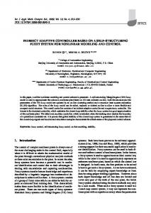
20 set of controllers (known as the multi-controller) which is supervised by a superior controller (supervisor) that compares the some estimates to the plant. A switching signal included in the supervisor chooses the best controller to control the process. This idea is presented in Figure 3.1.

Figure 3.1: Hybrid control concept

The supervisor controller consists of estimators (multi-estimator) that estimates each output of the n controllers plus observers. Each estimate is compared to the process output y. The multi-estimator is a set that describes a family M :=

[

Mp

(3.1)

p∈P

Mp := {x˙ p = Ap (xp , u, y), yp = Cp (p, xp , u, y) : p ∈ P}

(3.2)

where P is the set of estimators (E) and p is the number of the estimator. The state vector of the model set is xp , yp is the estimated vector of the pth estimator, u is the control vector and Ap and Cp are functions. The family of the estimators is M with Mp estimators. Controller switching is performed by a switcher that receives the switching signal σ from the supervisory control. Similarly to the multi-estimator, the controller set defines a family as C :=

[

Cq

(3.3)

q∈Q

Cq := {z˙ q = Fq (zq , y), u = Gq (zq , y) : q ∈ Q}

(3.4)

21 where Q is the set of controllers and q is the number of the controller. The state vector of the controller is zq with Fq and Gq being functions. The family of the controllers is C with Cq controllers. There is a process switching signal ρ which determines the selected control model in the supervisor. The switching signal σ from the supervisory control may be different from the signal ρ. Hence, there is a mapping σ = χ(ρ) ∈ Q, ρ ∈ P. This means that the controller number could be different from the observer number. This work assumes the mapping σ = ρ ∈ P ≡ Q which means that each ensuing pair is made up of one controller and one observer. The formal definition of a switched system is presented as follows.

Definition 3.1 Switched system − (HESPANHA, 2002). The switched system includes the process, controller set, and the estimator set x˙ = Aσ (x, w)

ep = Cp (x, w),

ρ∈P

(3.5)

(3.6)

where x denotes the state of the process and w is the disturbance. The supervisor possesses both process switching (PS) and switching logic (S) in order to generate the signal σ to switch to the best controller. Switching logic prevents chattering (high frequency of σ changing) of the switching signal. Process monitoring is presented in Figure 3.2, where yp is the output of the estimator p, ep is the error of the estimator p and µp is the monitoring signal of the estimator p.

Figure 3.2: Monitoring signal process

22

3.3

Supervisory Properties

To guarantee correct switching between controllers, Hespanha (2002) presented two important properties of the switching system: matching and detectability. The matching property means there is an estimator with output yp that provides a good approximation of the output of the process p. Detectability means that the switching system must be detectable with respect to ep for each controller χ(p) ∈ Q. These properties are summarized as Matching: a good approximation of yp needs to be provided by the multi-estimator, i.e., ep needs to be small whenever the process Mp ∈ M . Detectability: The error between the current and initial system states may be occasionally small, as long as system detectability is guaranteed, no matter what its initial state. Each estimator requires detectability related to the error estimator ep when a switching signal is fixed at σ = χ(ρ) ∈ Q.

Figure 3.3: Injected system in cascade (HESPANHA,2002)

The signal σ is generated by the switching logic. The switching control needs to have other properties such as small error and non-destabilization. Small error: For a process switching signal ρ which satisfies σ = χ(ρ), the boundedness of the error vector eρ must be guaranteed by the switching logic. The error vector eρ is the smallest sub-vector of the error vector ep under any norm. Non-destabilization: The system must be stable permanently in order to maintain detectability. Switching stopping in finite time can be guaranteed by means of a scale-independent hystere-

23 sis switching logic. This logic can be applied for linear and nonlinear observers and controllers.

3.4

Hysteresis Switching Logic

The error between the output yp of the estimators and the system output y is evaluated to select the best controller. The error vector ep is written as the difference between the estimate yp and the output y. The best controller has the smallest element of the error vector. However, the error vector can present with two or more of its entry close to each other. So, chattering can occur because two or more controllers could be selected. The scale-independent hysteresis switching logic guarantees that chattering will not occur and that the non-destabilization property is maintained (HESPANHA, 2002). Scale-independent hysteresis means that the switching signal will not change since the current monitoring signal µp will be less than others within certain comparative scales. The hysteresis logic diagram is presented in Figure 3.4. The monitoring signal vector µp is defined as follows Definition 3.2 Monitoring Signal − (HESPANHA, 2002). µ˙ p = −λµp + γ(kep k), p ∈ P

(3.7)

where λ denotes a constant non-negative forgetting factor, γ is a class K function (Lima (2009)) and k.k is any norm. The initial value of the monitoring signal is µ(0) > 0.

Figure 3.4: Scale-independent hysteresis switching logic (HESPANHA, 2002)

24 For the purposes of introducing the switching logic, let the positive constant of the hysteresis be h and consider the index of the minimum value of the µp that comes from arg min µp . The logic operates in the following way: start by taking ρ = arg min µp and do σ = ρ. When µρ 0.79 Nonlinear observer with notch filter 0.79 - 0.67 Nonlinear observer with notch filter 0.67-0.45 Nonlinear observer with notch filter < 0.45 Nonlinear observer for extreme seas

Table 5.2: Reference drafts for control model Reference Shuttle tanker FPWSO Draft k h [m] h [m] 1 8.00 21.00 2 12.48 18.21 3 17.50 15.42

57 y

y

Model for process for p=3

+-


+-


++-


+-


+-


+-


+-


u


yp


++-

m1

e1

Switching logic


++-

Monitoring sginal

y1


Supervisory control

ep

Switching signal s

mp

Multiestimator Controller and Observer y

u

Observer for s=1

Controller for k=1

Observer for s=2

Controller for k=1

Observer for s=3

Controller for k=1

Observer for s=4

Controller for k=1

Observer for s=1

Controller for k=2

Observer for s=2

Controller for k=2

Observer for s=3

Controller for k=2

Observer for s=4

Controller for k=2

Observer for s=1

Controller for k=3

Observer for s=2

Controller for k=3

Observer for s=3

Controller for k=3

Observer for s=4

Controller for k=3

Observer set

Controller set

Environment

Marine vessels

Command signal u

Switcher

Figure 5.1: Hybrid concept applied to offloading operation

Output y

58 As presented in Chapter 3, the mapping is σ = ρ and, as a consequence, P ≡ Q. Table 5.3 presents a mapping between the multi-estimator, the draft ranges and sea states for reference purposes. To simplify the reference, the multi-estimator is denoted by p, the sea states ranges are denoted by s = 1, ..., 4 as defined in Table 5.1, and draft ranges are denoted by k = 1, ..., 3 as defined in Table 5.2. To monitor sea state, the motion peak-frequency is assumed to be slowvarying, i.e., ω˙ p = 0 (DONG, 2005), and its estimate is calculated as presented in Section 5.4. The offloading operation between DP vessels takes around 24h. Then, their drafts are assumed ˙ ≈ 0, where h = [ h h ]T are the drafts for FPWSO and the shuttle to be slow-varying, i.e., h 1 2 tanker, respectively.

Table 5.3: Mapping between supervisor and controller set Multi-estimator p=q 1 2 3 4 5 6 7 8 9 10 11 12

Sea state ranges s 1 2 3 4 1 2 3 4 1 2 3 4

Draft ranges k 1 1 1 1 2 2 2 2 3 3 3 3

The switching controller possesses a controller set based on the geometric control law and the nonlinear observer. PD-like controller is also studied using the same observer. The switching control model for the offloading operation is presented in the following sections. The multiestimator and the controller and observer sets that comprise the switching control are presented. Finally, the peak-frequency tracker, draft survey calculation and supervisory tuning are all discussed.

59

5.2

Nonlinear Observer Set and Multi-estimator

The observer set and multi-estimator for the hybrid control presented here are based on the indices in Table 5.3.

5.2.1

Multi-estimator with Wave-Frequency Model

The nonlinear observer with wave-frequency motion model was proposed in Section 4.2.1. This observer is applied to three of the four sea state ranges of the switching controller (s = 1, ..., 3). So, nine estimators of the supervisory control are based on the nonlinear observer model (p = {1, ..., 12} − {4, 8, 12}). Considering Section 4.2.1, an extended system model is written as ξ˙ = Ωξ + Σw

(5.1)

η˙ = J (ψ 1 , ψ 2 )ν

(5.2)

b˙ = −T −1 b + Ψn

(5.3)

M k ν˙ + D k ν = J T (ψ 1 , ψ 2 )b + τ c

(5.4)

˙ = 02×1 h

(5.5)

ω˙p = 0

(5.6)

y=

(η + Γξ)T

hT

ωp

T

(5.7)

where M k and D k denote the matrices calculated in draft range k. This model is similar to the system model presented by Dong (2005) except for the inclusion of (5.5). Dong (2005) took the peak-frequency to be slow-varying, i.e., ω˙p = 0. Here, the drafts are also assumed to be ˙ = 0. Thus, the output vector is y ∈ R9 with the extended system model slow-varying, i.e., h

60 having draft vector h. A system can be expressed concisely using (5.1) to (5.7) as x˙ p = Ap xp + B q τ q + E p w

(5.8)

y = C p xp

(5.9)

where the state vector is xp = [ ξ T is w = [ wT

bT

ηT

T 33 ω p ] ∈ R and the disturbance vector

hT

νT

T 12 6 33×33 , B ∈ q nT ] ∈ R . The control vector is τ q ∈ R . The matrices Ap ∈ R

R33×6 , E p ∈ R33×12 and C p ∈ R9×33 are written as Ap =

Ω 021×12

012×21 ALF

Bq =

Ep =



Γ

C p =  02×6 01×6

012×6 B LF

(5.10)

(5.11)

Σ12×6 012×6 021×6 E LF

(5.12)

 I 6×6 06×6 06×6 06×2 06×1 02×6 02×6 02×6 I 2×2 02×1  01×6 01×6 01×6 01×2 1

(5.13)

The matrices ALF ∈ R21×21 , B LF ∈ R21×6 , E LF ∈ R21×6 are written as qi q  ALF

  =  

06×6 06×6 J (ψ1 , ψ2 ) −1 06×6 −T 06×6 06×6 06×6 −Mk−1 D k 02×6 02×6 02×6 01×6 01×6 01×6  B LF

  =  

 E LF

  =  

06×6 06×6 Mk−1 02×6 01×6



06×6 Ψ 06×6 02×6 01×6



    

    

06×2 06×2 06×2 I 2×2 01×2

06×1 06×1 06×1 02×1 1

     

(5.14)

(5.15)

(5.16)

61 This system model is used as the estimator model for the wave-frequency motion of the switching control. So, the estimator is constructed similarly to the state observer as presented in Section ˆ p can be written as 4.2.1. Considering (5.1) to (5.6), the state observer vector x ˆ˙ p = Ap x ˆ p + B q τ q + K ps (y − yp ) x

(5.17)

ˆp yp = C p x

(5.18)

ˆp = where the state observer vector is x

T

ξˆ

η ˆT

T

ˆ b

ν ˆT

ˆ h

T

T ω ˆp

∈ R33 . The vector

yp ∈ R9 is the output of the state observer of the process p (see Figure 5.1). The frequency ω ˆ p is the peak-frequency spectrum obtained from the spectra analysis (see Section 5.4) and the ˆ is obtained from the draft survey calculation (see Section 5.5). Matrix estimated draft vector h K ps ∈ R33×9 is written as K ps =

K 1s K LFs

012×2 012×1 021×2 021×1

(5.19)

where K 1s ∈ R12×6 and K LFs ∈ R21×6 . Matrix K LFs ∈ R21×6 is written as  K LFs

  =  

K 2s K 3s K 4s 02×6 01×6

     

(5.20)

with the matrices K 2s , K 3s and K 4s ∈ R6×6 being presented in Section 4.2 and calculated as presented by Fossen and Strand (1999). Each matrix with index s is calculated for sea state range s.

5.2.2

Multi-estimator for Extreme Seas

The nonlinear observer for extreme seas was presented in Section 4.2.2. This model is applied to one of the four sea state ranges of the switching control when s = 4. So, three estimators of the supervisory control use this nonlinear observer model (p = {4, 8, 12}). Consider the following

62 system model for extreme seas

η˙ T = J (ψ1 , ψ2 )ˆ νT

(5.21)

b˙ T = −T −1 bT + Ψn

(5.22)

M k ν˙ T + D k νT = J T (ψ 1 , ψ 2 )bT + τ c

(5.23)

˙ = 02×1 h

(5.24)

ω˙p = 0

(5.25)

The output vector y ∈ R9 is written as y=

η TT

hT

ωp

T

(5.26)

Similarly to the previous section, the model is concisely written as x˙ p = Ap xp + B q τ q + E p w

where the vector xp = [ η TT

bTT

ν TT

hT

(5.27)

T 21 21×21 , B = B p LF ∈ ω p ] ∈ R , Ap = ALF ∈ R

R21×21 in (5.15) and Ep = ELF ∈ R21×21 . The disturbance vector is w = n ∈ R6 . The system model presented is the switching control estimator model for extreme seas. The switching control estimator is constructed similarly to the state observer as presented in Section 4.2.2. Based on ˆ p can be written as (5.21) to (5.25), the state observer vector x

ˆp = where x

η ˆTT

T ˆ bT

ν ˆTT

ˆ˙ p = Ap x ˆ p + B q τ q + K ps (y − yp ) x

(5.28)

ˆp yp = C p x

(5.29)

ˆ h

T

T ω ˆp

∈ R21 . The matrix Cp ∈ R9×21 is written as



 I 6×6 06×6 06×6 06×2 06×1 C p =  02×6 02×6 02×6 I 2×2 02×1  01×6 01×6 01×6 01×2 1

(5.30)

63 The matrices K2T s , K3T s and K4T s ∈ R6×6 that compose Kp s are similar to the estimator model for wave-frequency motion.

5.3

Controller Set

The geometric control law is used into the supervisory switching controller set. For the sake of comparison, the PD-like control law is also studied. Both geometric and PD-like controllers are determined for the vessels’ dynamic positioning systems in offloading operations, as presented in Sections 4.4.2 and 4.4.4, respectively. The current section describes both control laws employed when selecting the switching controller. The control laws take into account the estimated values of positions and headings, and velocities and external forces. For each controller, two state observers are considered, i.e., with and without wave-frequency vessel motions.

5.3.1

Geometric Controller Set

In order to present the geometric control law for the nonlinear observer with the wave-frequency model, the control law is indexed from (4.96) and yields ˙ ηˆ˙ + W ˙ r x˙ r + W r x uGp = −ˆ b + (D ηˆ − J M k J J˙ J T )η ˆ˙ − M ηˆW −1 (W ¨r + v p )

(5.31)

where uGp ∈ R6 is the control vector for p = {1, ..., 12} − {4, 8, 12}. τ qi = J (y)T uGi = −J (y)T ˆ b + (D k − M k J (y)J˙ (y))ˆ ν− (5.32) ˙ J (y)ν + W ˙ r x˙ r + W r x −M k J (y)−1 W −1 (W ¨r + v i ) v i = K pk .C (ˆ η , xr ) + K dk .C˙(ˆ η , xr )

(5.33)

˙ , W r and W ˙ r The matrices D ηˆ and M ηˆ are defined in Section 4.3.2. The matrices W , W are defined in Section 4.3.2. The new control vector is v i ∈ R6 . The positioning constraint is C (ˆ η , xr ) and is presented in (4.80).

64 The gain matrices K p ∈ and K d ∈ R6×6 are defined as K pk = diag{ ωn2 1

K dk = 2.diag{ ςcn1 ωn1

... ωn2 6 }

... ςcn6 ωn6 }

(5.34)

(5.35)

where ςcni and ωni are control parameters. For control laws with p = {4, 8, 12}, the geometric law is presented as follows τ qi = −J (y)T ˆ bT + (D k − M k J (y)J˙ (y))ˆ νT − (5.36) ˙ J (y)ν T + W ˙ r x˙ r + W r x −M k J (y)−1 W −1 (W ¨r + vT i ) vT i = K pk .C (ηˆT , xr ) + K dk .C˙(ηˆT , xr )

(5.37)

where the gain matrices K p and K d are the same as in (5.34) and (5.35), respectively. Other matrices and the constraint in (5.36) and (5.37) are calculated for xpi for i = {4, 8, 12}.

5.3.2

The Proportional and Derivative Controller Set

The proportional and derivative controller with p = {1, ..., 12} − {4, 8, 12} is presented as follows uP Di = K pk e ˆ˙ − ˆ b ˆ + K dk e

(5.38)

τ qi = J (y)T uP Di

(5.39)

where uP Di ∈ R6 is the control vector. The matrix K pk ∈ R6×6 is the proportional control gain matrix and K dk ∈ R6×6 is the derivative control gain matrix defined as K pk = M k .diag{ ωn2 1

K dk = 2.M k .diag{ ςcn1 ωn1

... ωn2 6 }

... ςcn6 ωn6 } − D k

(5.40)

(5.41)

where ςcni and ωni are control parameters. The error vector and its time-derivative are written

65 as e ˆ = [ˆ η − ηr ]

(5.42)

e ˆ˙ = [J (y)ˆ ν − η˙ r ]

(5.43)

where e ˆ and e ˆ˙ ∈ R6 . For the control laws for i = {4, 8, 12}, the PD-like control law is presented as follows ˆT + K dk e ˆ˙ T − ˆ bT uP Di = K pk e

(5.44)

where the gain matrices K p and K d are the same as in (5.40) and (5.41), respectively. The error vector and its time-derivative are written using the estimates from the nonlinear observer for extreme seas as follows

5.4

e ˆ = [ˆ ηT − ηr ]

(5.45)

e ˆ˙ = [J (y)ˆ ν T − η˙ r ]

(5.46)

Peak-Frequency Tracker

Vessel motion peak-frequency of the vessel motions is used to estimate the wave-frequency motion in the measurement signal. This peak-frequency motion does not necessarily correspond to sea spectrum peaks. However, the differences in values are negligible and can be ignored. This is evaluated in Appendix C. In order to estimate motion peak-frequency ωp , a spectrum estimate of the vessel motion is made during the simulations. A fixed data (window of the motion is recorded and the motion spectra of surge, sway and yaw of the vessels is evaluated. To improve spectrum analysis, a cascaded high-pass frequency filter is applied to the motion measurement. This filter is given by

ψhf (s) =

nf Y

Tf .s 1 + Tf .s

(5.47)

66 where ψhf (s) is the transfer function of the high-pass frequency filter, Tf is the cut-off highfrequency and nf is the number of the filters in cascade. A more detailed analysis can be found in Fossen (1994). Figure 5.47 presents the spectra of ST surge motion comparing cascaded high-pass frequency filters with different orders.

Figure 5.2: Spectrum analysis of the Cascaded High-Pass Frequency Filter

Figure 5.47 shows that the higher the filter order, the lower the low-frequency peak which greatly facilitates high frequency peak detection. During simulations, filter order is n = 10. The peakfrequency is obtained from the average surge and sway peaks of both vessels. Yaw motion is not included because, even applying the cascaded filter, the estimate of the frequency ωp is not accurate enough.

5.5

Draft Survey Monitoring

Draft variation during offloading is taken into account by the supervisory control. The multiestimator uses vessel drafts to estimate the error vector epi of the process i. Vessel draft can be calculated by a draft survey calculation since oil transfer flow between vessels is known. Hence, if the draft is known during the offloading operation, the inertia properties can be estimated. Here, the trim and heel are assumed to be null. See Appendix A for more details about inertia

67 properties.

5.6

Supervisory Control Tuning

The chattering that can occur during the change of control law and state observer is avoided by means of the switching logic hysteresis. The hysteresis parameter h needs to be chosen correctly in order to neither freeze switching if the value h is too high, nor cause chattering if the value h is too low. B¨ oling, Seborg and Hespanha (2005) appropriately choose the forgetting factor λ so as to avoid impulsive or slow behavior of µp . Previous simulations evinced positive results for the scale-independent hysteresis switching logic µp = 1/10, hysteresis h = 20% and a data window of 500s interval to generate motion spectra.

68

Chapter 6 Simulation Results

6.1

General

Hybrid concept performance as applied to an offloading operation is evaluated through simulation of some scenarios from Brazilian waters. A typical environmental scenario is presented in Figure 6.1. The current flows south (S) and its velocity range is 0.1-0.7m/s. This velocity range and incidence angle represent 99% and 33% of the occurrence, respectively. The wind and waves (local sea) come from the northeast direction (NE). This direction represents a little more than 30% of the direction occurrence.

North Uc = 0.1 - 0.7 m/s (99%) S (33%)

Uw = 4.0 - 15.0 m/s NE (33%) Hs = 0.1 – 2.5 m (97%) Tp = 4.0 – 10.0s NE (31%)

d

East

West

Y1

Y2

vessel reference

South

Figure 6.1: Typical environmental conditions for Brazilian basin

69 Figure 6.1 also presents the significant wave height, wave-frequency peak and wind velocity ranges. Due to the difference between the incidence angles of the wind/wave and current, a convenient reference for the heading of the vessels is between 0◦ and 45◦ . To analyze controller performance under different environmental scenarios and references, five simulation cases are considered as follows:

• Case 1: Analyze controller performance due to a change in the position reference; • Case 2: Evaluate the positioning of the vessels due to the changes in their relative distance; • Case 3: Evaluate the consequence, in terms of relative positioning, when an extra force acts on the FPWSO only; • Case 4: Test switching control in transitions from calm environmental scenarios to gradually harshening; • Case 5: Test switching control in transitions from harsh environmental scenarios to gradually becoming calm; • Case 6: Assess controller performance during a day-long operation when the environmental scenario is harshening.

Both geometric controller and PD-like controller are considered. For the cases 1 to 5, the controllers’ parameters are tuned to three different drafts (reference drafts from perturbation model - see Figure 6.2). To evaluate the performance of these controllers, simulations are carried out using constant drafts set for these reference drafts. The observers’ parameters are selected by the supervisory control. The case 6 is a realistic scenario where the drafts vary and the observer/controller parameters are automatically selected by the supervisory control.

Figure 6.2: Reference Draft for the vessels

70 Table 6.1 and Table 6.2 present the references for the vessels and the parameters of the environmental scenarios, respectively.

Table 6.1: Reference for simulations

Table 6.2: Scenarios for simulations

6.2

Case 1: Reference Change

This section presents simulation results that tests controller performance when the reference is changed. The environmental scenario for these simulations is presented in Figure 6.3. The sea state condition is kept constant and the observer parameters are selected by the supervisory control and they are equal to the first range of the peak frequency motion (calm sea). The heading references for FPWSO and the shuttle tanker are modified from 10◦ to 0◦ . To maintain the alignment with the FPWSO, the shuttle tanker has its reference changed.

71

North

North

Y2 = 0°

vessel reference

constant drafts

South

Time = 4.000s

East

d = 150m

Y2 = 10°

vessel reference

Hs = 1.5m Tp = 4.8s Uw = 10.0 m/s NE

ST

d = 150m

Y1 = 0°

West

Hs = 1.5m Tp = 4.8s Uw = 10.0 m/s NE

East

West

Y1 = 10°

FPWSO

Uc = 0.7 m/s S

Uc = 0.7 m/s S

constant drafts

South

Figure 6.3: Environmental conditions and first maneuver

Geometric controller achieves the reference and maintains the vessels in their correct positions and headings as presented in Figures 6.4. The relative distance is also maintained by the controllers for each draft as seen in Figure 6.6. PD-like controller also achieves the reference and maintains the vessels’ positioning and relative distance as presented in Figure 6.5.

72

Figure 6.4: Positioning using Geometric Controller

73

Figure 6.5: Positioning using PD-like Controller

74

Figure 6.6: Distance between vessels

Estimates velocities are well-estimated by the nonlinear observer with wave-frequency model because they converge to real values, with the exception of the estimated surge velocity of the shuttle tanker as presented in Figures 6.7 and 6.8. As discussed in Appendix C, the surge motion of the shuttle tanker can exhibit a bimodal spectrum response. The cut-off frequency of the nonlinear observer is always tuned for the highest peak-frequency of the spectrum. So, the second peak with the lowest energy amplitude could not be filtered properly. Consequently, some wave-frequency motion appears in the surge control force of the shuttle tanker. The observer filters the wave-frequency motion when final draft is set better than other drafts. Despite the fact that the surge motion presents some wave-frequency influence, overall positioning is carried out correctly.

75

Figure 6.7: Vessel velocities using Geometric Controller

76

Figure 6.8: Vessel velocities using PD-like Controller

77

Figure 6.9: External forces using Geometric Controller

External forces estimates from Markov process converge to values approximating to the real external forces in terms of magnitude and frequency as shown in Figures 6.9 and 6.10.

78

Figure 6.10: External forces using PD-like Controller

The geometric control law is presented in Figure 6.11. PD-like control law (Figure 6.12) is similar to this control law. Wave-frequency motion appears on surge control law of the shuttle tanker as position estimate was not filtered properly. The performance of the controllers is good because the matrices M and D are set for the draft simulated. When offloading is taking place, the performance tends to deteriorate until the hybrid control switches the controller parameters.

79

Figure 6.11: Control forces using Geometric Controller

80

Figure 6.12: Control forces using PD-like Controller

81

6.3

Case 2: Distance Change

The simulation results that tests controller performance when the distance between vessels is changed are presented. The environmental scenario for these simulations is presented in Figure 6.13. Sea state condition is constant and the observer parameters are selected by the supervisory control and they are equal to the fourth range of the peak frequency motion (extreme sea). Distance between the vessels is altered from 150.0m to 200.0m. North

North

d1 = 150m

Y1 = 10°

West

Hs = 2.0m Tp = 17.0s Uw = 10.0 m/s NE

East

West

Y1 = 10°

Y2 = 10°

vessel reference

d2 = 200m

Y2 = 10°

vessel reference

constant drafts

South

Hs = 2.0m Tp = 17.0s Uw = 10.0 m/s NE

East

Uc = 0.7 m/s S

Uc = 0.7 m/s S

Time = 1h

constant drafts

South

Figure 6.13: Environmental conditions and second maneuver

The geometric control law is presented in Figure 6.14. PD-like control law is similar to this control law and it is presented in Figure 6.15. The relative distance is also maintained by the controllers for each draft as seen in Figure 6.16. The shuttle tanker heading presents with a different value from the heading set-point. This error occurs because the external forces and moment on the vessel are close to maximum thruster capability.

82


83


84


Vessel motions present the wave-frequency motion influence (Figures 6.14 and 6.15) as well as the velocity estimates do it (Figures 6.17 and 6.18). However, the yaw velocities and headings for both vessels do not to evince this frequency influence on yaw motion due to their high yaw inertia mainly in the final draft case.

85


86


Both estimated external forces and moments (see Figures 6.19 and 6.20) and control laws (see Figures 6.21 and 6.22) undergo wave-frequency influence. In spite of this wave-frequency motion influence and some control saturation, both geometric and PD-like controllers are able to maintain positioning and the relative distance for each draft simulated.

87


88


89


90


91

6.4

Case 3: Occurrence of an Extra Force

Although controllers’ performance has been very similar so far, when some event happens to the FPWSO and does not occur with the shuttle tanker, a small difference can be found. For instance, if a strong wind blast reaches the FPWSO and does not affect the shuttle tanker, some movement of the FPWSO is to be expected. This can happen because the height of the FPWSO and its exposed area to wind, with respect to water level, are both greater than those of shuttle tanker. As discussed in Chapter 4, if the PD-like controller is applied with the error e, the set-point of the shuttle tanker is not altered even if the FPWSO moves from its set-point. The geometric controller is applied using the constraint as output and if the FPWSO moves from her set-point, the ST also moves. To evaluate this behavior, simulations with an additional force to the FPWSO are performed. The environmental scenario for this simulation is presented in Figure 6.23. The sea state condition is kept constant and the observer parameters are selected by the supervisory control and they are equal to the first range of the peak frequency motion (calm sea). The extra force is inserted in the interval of 1.500s to 2.500s.

North

North

d1 = 150m

Y2 = 10°

vessel reference

d1 = 150m Extra force on FPWSO

Y2 = 10°

vessel reference

constant drafts

South

Hs = 2.0m Tp = 8.0s Uw = 10.0 m/s NE

Y1 = 10°

West

Hs = 2.0m Tp = 8.0s Uw = 10.0 m/s NE

East

West

Y1 = 10°

Time = 4.000s

East

Uc = 0.7 m/s S

Uc = 0.7 m/s S

constant drafts

South

Figure 6.23: Environmental conditions and third maneuver

Vessels’ positioning are maintained for both controllers even after the extra force occurrence appears or ceases as presented in Figures 6.24 and 6.25. The difference between the controllers

92


is the shuttle tanker positioning. As discussed, the geometric controllers acts upon the shuttle tanker to maintain the relative distance and the PD-like controller does not act upon it.

93


94


The simulations show that the distance error is small between both controllers’ results when the extra force is inserted into it (peak after 1.500s) and the force ceases (peak around 2.500s). In spite of this small error difference, the error amplitude is negligible and the controllers can be consider similar. Velocities are well-estimated by the nonlinear observer with wave-frequency model, with the exception of the estimated surge velocity of the shuttle tanker as presented in Figures 6.27 and 6.28. This behavior is the same one discussed in Section 6.2. The nonlinear observers estimates using the geometric controller present some estimated velocity peaks due to change in shuttle tanker reference.

95


96


97


Estimation of the external forces and moment depend on the control law considered. This dependence is due to the shuttle tanker reference that is changed only in the case of PD-like controller. So, an external force and moment difference can be found between the controllers as presented in Figures 6.29 and 6.30. Obviously, both controller have different actions that make the shuttle tanker moves in the case

98


of geometric controller and do not move it in the case of the PD-like controller. Control forces peaks appear in the ST geometric control forces as in Figure 6.31 that does not appear in the ST PD-like control forces as presented in Figure 6.32. This occurs due to difference between the geometric controller constraint and PD-like error.

99


100


101

6.5

Case 4: Harshening Sea State

Simulations are carried out to evaluate the switching control when the sea state is harshening. The environmental scenario for these simulations is presented in Figure 6.33. The direction of the current and wind are kept constant. The direction of the waves and the significant wave height Hs are also kept constant excepting the value of the peak period T p. The peak period of the waves varies from 4.5s to 15.0s. The switching signal σ and the estimated peak frequency ω ˆ p are now calculated.

North

North

d1 = 150m

Y1 = 10°

West

Hs = 2.0m Tp = 4.5s Uw = 10.0 m/s NE

East

West

Y1 = 10°

Y2 = 10°

vessel reference

Hs = 2.0m Tp = 15.0s Uw = 10.0 m/s NE

d1 = 150m

East

Uc = 0.7 m/s S

Uc = 0.7 m/s S

Y2 = 10°

vessel reference

constant drafts

South

Time = 4.000s

constant drafts

South

Figure 6.33: Environmental conditions and forth maneuver

Vessels’ positioning and the relative distance are maintained for both controllers during the simulation with the sea condition variation as presented in Figures 6.34, 6.35 and 6.36. Wavefrequency motion influence on the position and heading estimates was expected due to the nonlinear observer parameter changes.

102


103


104


The velocity estimates made by the nonlinear observers are good because they converge to real values as presented in Figures 6.37 and 6.38, even if its parameters are changed by the switching controller. The wave-influence motion influence is filtered from the estimated velocities as presented in those figures excepting for t > 3.500s.

105


106


107


The external force estimates made by the nonlinear observer are also good as presented in Figures 6.39 and 6.40 in spite of some magnitude errors. The effect of the nonlinear observer for extreme seas on the external force estimates can be seen in those figures for t > 3.500s.

108


109


Geometric control law is very similar to PD-like control forces as presented in Figures 6.41 and 6.42.

110


111 During these simulations, the estimated peak frequency of the motion spectrum is lose to real values as presented in Figure 6.43. Hence, the switching control generates the switching signal σ, correctly selecting the nonlinear observer associated with estimated peak frequency as presented in Figure 6.43. Therefore, the estimates of the positions and headings for both vessels has filtered the wave-frequency motion influence. Obviously, this filtering process does not happen when the the nonlinear observer for extreme seas is selected (t > 3.500s). The switching control takes 500s to change the nonlinear observer. This interval is the time difference between the change of the peak period T p and the change in the switching signal σ. It is the maximum time in which the signal σ is updated because it is the length of the data window for generating the motion spectrum of the vessels. Despite the delay in switching the observer, the switching control changes the observer parameters correctly. Vessels’ positioning are maintained in their set-points for both geometric and PD-like controllers, and for each draft simulated.

112

Figure 6.43: Peak Estimation and σ

113

6.6

Case 5: Sea State Becoming Calm

The simulations are carried out to evaluate the switching control when the sea state is getting calm are presented. The environmental scenario for these simulations is presented in Figure 6.44. The direction of the current and wind are kept constant. The direction of the waves and the significant wave height Hs are also kept constant excepting the value of the peak period T p. The peak period of the waves varies from 15s to 4.5s. The switching signal σ and the estimated peak frequency ω ˆ p are now calculated.

North

North

d1 = 150m

Y2 = 10°

vessel reference

d1 = 150m

Y2 = 10°

vessel reference

constant drafts

South

Hs = 2.0m Tp = 4.5s Uw = 10.0 m/s NE

Y1 = 10°

West

Hs = 2.0m Tp = 15.0s Uw = 10.0 m/s NE

East

West

Y1 = 10°

East

Uc = 0.7 m/s S

Uc = 0.7 m/s S

Time = 4.000s

constant drafts

South

Figure 6.44: Environmental condition and fifth maneuver

Vessels’ positioning and the relative distance are maintained for both controllers during the simulation with the sea condition variation as presented in Figures 6.45, 6.46 and 6.47. As the previous section, some wave-frequency motion influence was expected on the position and heading estimates.

114


115


116


The estimates made by the nonlinear observer are good as presented in Figures 6.48 and 6.49, even if its parameters are changed by the switching controller. The wave-influence motion filtering on the can be seen in those figures excepting for t < 500s.

117


118


119


The external force estimates made by the nonlinear observer are also good as presented in Figures 6.50 and 6.51. The effect of the nonlinear observer for extreme seas on the external force estimates can be seen in those figures for t < 500s.

120


121


Geometric control law is very similar to PD-like control law as presented in Figures 6.41 and 6.42.

122


123 During these simulations, the peak frequency of the motion spectrum is close to real values as presented in Figure 6.54. Hence, the switching control generates the switching signal σ, correctly selecting the nonlinear observer associated with estimated peak frequency as presented in Figure 6.54. Therefore, the estimates of the positions and headings for both vessels has filtered the wave-frequency influence. Obviously, this filtering process does not happen when the the nonlinear observer for extreme seas is selected (t > 3.500s). As discussed in the previous section, the switching control takes 500s to change the nonlinear observer. The switching control changes the observer parameters correctly. Vessels’ positioning are maintained in their set-points for both geometric and PD-like controllers, and for each draft simulated.

124

Figure 6.54: Peak Estimation and σ

125

6.7

Case 6: Day-long Operation Simulation

A day-long simulation is carried out to evaluate the switching control for a complete offloading operation. At simulation outset, the FPWSO has full draft and the shuttle tanker has ballast draft. The environmental scenario is presented in Figure 6.55. Sea state is associated with the wind similar to that to be found in Brazilian waters. In this simulation, sea state is harshening as such waves and wind parameters are changing. Current velocity and direction are kept constant.

North

North

d1 = 150m

Y2 = 10°

vessel reference

d1 = 150m

Y2 = 10°

vessel reference

varying drafts

South

Hs = 2.5m Tp = 14.0s Uw = 15.0 m/s NE

Y1 = 10°

West

Hs = 1.0m Tp = 4.0s Uw = 4.0 m/s NE

East

West

Y1 = 10°

East

Uc = 0.7 m/s S

Uc = 0.7 m/s S

Time = 1 day

varying drafts

South

Figure 6.55: Environmental conditions and sixth maneuver

The positioning of the vessels are maintained as desired by both controllers as presented in Figures 6.56 and 6.57 (geometric controller) and Figures 6.58 and 6.59 (PD-like controller). The relative distance between vessels is also maintained around 150m as presented in Figure 6.60.

126

Figure 6.56: FPWSO positioning: geometric controller

127

Figure 6.57: Shuttle tanker positioning: geometric controller

128

Figure 6.58: FPWSO positioning: PD-like controller

129

Figure 6.59: Shuttle tanker positioning: PD-like controller

130


131 The nonlinear observer filters the wave-frequency motion from the positions and heading for both vessels (see Figure 6.57 to 6.60). The nonlinear observers for the wave-frequency model are selected from t = 0h to t = 16h. The nonlinear observer for extreme seas is selected by the supervisory controller when t > 16h. The velocities estimates are close to the real velocities as presented in Figures 6.61 and fig:6.62 (geometric controller) and Figures 6.63 and 6.64 (PD-like controller).

132

Figure 6.61: FPWSO velocities: geometric controller

133

Figure 6.62: Shuttle tanker velocities: geometric controller

134

Figure 6.63: FPWSO velocities: PD-like controller

135

Figure 6.64: Shuttle tanker velocities: PD-like controller

136

Figure 6.65: FPWSO external forces: geometric controller

External force estimates converge to the real values as presented in Figures 6.65 and fig:6.66 (geometric controller) and Figures 6.67 and 6.68 (PD-like controller).

137

Figure 6.66: Shuttle tanker external forces: geometric controller

138

Figure 6.67: FPWSO external forces: PD-like controller

139

Figure 6.68: Shuttle tanker external forces: PD-like controller

140

Figure 6.69: FPWSO control forces: geometric controller

Control laws calculated by both controllers are very similar to each other as presented in Figures 6.69 and fig:6.70 (geometric controller) and Figures 6.71 and 6.72 (PD-like controller).

141

Figure 6.70: Shuttle tanker control forces: geometric controller

As discussed in Chapter 4, the controllers can be considered similar and as well as the switching controller.

142

Figure 6.71: FPWSO control forces: PD-like controller

143

Figure 6.72: Shuttle tanker control forces: PD-like controller

144 The evolution of the sea state and the wind are presented in Figure 6.73. During the offloading operation, the switching controller is monitoring the peak frequency of the motion spectrum. The estimated peak frequency is close to the real peak frequency as presented in Figure 6.73. Drafts vary during the simulation and are assumed to be known (see Figure 6.73). So, the switching signal is switched to select the best observer/controller for the draft vector h and peak frequency ωp pairing. The switching signal σ in Figure 6.73 is presented together with the arrows that indicate the intervals where the three reference drafts and the four sea state ranges can be found. Switching signal change is correct in accordance with Table 5.3. This means that the best observer/controller is selected for the draft vector and peak frequency pairing. So, the switching controller works as designed.

145

Environment scenario

Hs [m]

2.5 2 1.5 1

0

2

15 Tp [s]

4

6

8

10

12

14

16

calm to extreme sea

calm sea

18

20

22

24

extreme sea

10 5 0

0

2

4

6

8

10

0

2

4

6

8

10

12

14

16

18

20

22

24

12 14 16 t [h] Frequency peak estimation

18

20

22

24

Uw [m/s] U

15 10 5

p [rad d/s]

0

Estimate Wave

1.5 1 0.5 0

2

4

6

8

10

12

14

16

18

20

22

24

Draft [m m]

20 15 FPWSO ST

10 0

2

4

6

8

10

ref. draft 1

12

14

16

18

ref. draft 2

20

22

24

ref. draft 3



10 5 0

sea1 0

2

4

sea2 6

8

10

sea4

sea3 12 t [h]

14

16

18

20

Figure 6.73: Environment, drafts, ωp and σ

22

24

146

6.8

Discussion and Conclusions

In the case of reference and the distance simulations, the geometric controller is able to maintain vessel positions and headings with a similar degree of accuracy to that of the PD-like controller. As discussed in Section 4.4.4, geometric control and PD-like controller performance are very similar when the vessels move slowly and the reference is constant. The main difference between the controllers is the inclusion of reference in the geometric control law. However, the control laws is very similar because of slow vessel velocities and constant reference. A small difference in the performance of the controllers appears when some unexpected event occurs for the FPWSO. In this case, the geometric controller moves the shuttle tanker and the PD-like controller does not. This is so because the geometric control, with the linearized output equal to the constraint, alters shuttle tanker set-point when the FPWSO leaves its set-point. The PD-like controller has constant vessel set-point of the vessels constant and so does not control the relative distance between the vessels as the geometric control does. Despite this difference, the amplitude of that distance error is small and the controllers can be considered similar. During simulations where sea conditions change constantly, the switching control chooses the correct nonlinear observer. Hence, the switching control operates correctly. The simulations present a maximum hanging lag of 500s. This delay is the data window formation spectrum generating and, as such, the maximum time for updating the parameters of the nonlinear observer. Data windows shorter than 500s are not enough to extract precise frequency motion estimate from the motion spectrum. This is the case because the vessels have a high inertia and their dynamics filter the wave-frequency motion to some extent. Where the one day simulation is concerned, the switching control makes the correct nonlinear observer and controller choices based on estimated peak frequency motion and the vessel drafts. This switching meets maximum error criterion imposed by the perturbation model. Nonlinear observer parameters are set for the highest peak frequency of the motion spectrum. Some response spectra analyzed in Appendix C present with a bimodal response. Consequently, for those periods of a day-long simulation when the bimodal response is present, the nonlinear

147 observer is not able to filter both peak frequencies. This occurs because the bandwidth of the filter does not include the second peak frequency and the observer does not suppress this frequency appropriately. This problem could be resolved by means of a fourth-order wavefrequency model whose bimodal response approximates the sea spectrum.

148

Chapter 7 Final Conclusions and Further Research

7.1

Final Conclusions

The main purpose of this work was to design a new integrated control strategy for the hybrid system to act upon a multibody system consisting of two dynamically positioned vessels. The vessels are the FPWSO and the shuttle tanker that carry out an offloading operation in tandem configuration. This control strategy ensures vessels remain within a relative distance of each other to avoid collision or excessive hawser tension. The hybrid controller takes into account variations in vessel draft and vessel motion peak-frequency as they may influence controller performance. Integrated control making use of geometric theory for dynamically positioned vessels is feasible. Establishing relative positioning is an intuitive way to generate a output system for the control strategy. The geometric controller can be implemented by means of an output linearization procedure. The idea is simple in spite of the sophisticated mathematics involved in the differential geometry. The switching control structure takes into account variations in some system parameters. There is some difficulty to allow for in tuning switching logic parameters in order to guarantee correct switching as there is no procedure to tune them, and they have been derived

149 from previous numerical simulations. When some major event, such as wind blast, impacts upon the FPWSO, it can lose its positioning and the shuttle tanker will follow the FPWSO because of their integrated control law. However, the same hybrid structure can take into account controllers with no integrated output which would be selected in the case of a major event. Another important factor to be considered is the availability of heading and position information. The integrated controller needs to have the vessels’ position measurement and to send the command to the thrusters of both vessels in real-time which, in practical terms, is a technical limitation.

7.2

Further Research

Suggestions for further research would include:

• The hybrid control presented assumes an initial FPWSO draft as this vessel can begin her operation in different drafts. The hybrid control would be able to set a variety of initial FPWSO drafts. This would result in an increased estimator number. • Thruster saturation can be interpreted as a hybrid dynamical system with three different dynamics: vessel dynamics in combination with thrust upper limit, intermediate (no saturation) and thrust lower limit. The switching control could take into account these new combined dynamics and, by means of the injected systems, system stability with thruster saturation could be proved; • The nonlinear observer model could be extended to consider a fourth-order wave-frequency model in order to approximate a bimodal vessel motion spectrum; • Side-by-side oil transfer could be controlled by hybrid and geometric means. Dynamics can account for the low speed of both vessels and their relative distance is maintained by the constraint geometric controller. Draft variation during oil transfer would be allowed for the hybrid control approach; • The hybrid controller could incorporate observer models that estimate both peak-wavefrequency vessel motion and wave direction. Vessel set-point could be changed depending

150 on wave direction; • Should DPS damage, such as drive-off, drift-off or black-out occur, the hybrid control would be able to take decoupled control laws into account; • New constraints could be established to restrict maximum vessel deviation from set-point. For instance, a maximum FPWSO radius could be assumed and a constraint could be described by placing a logarithmic function into the geometric controller.

151

References AARSET, M. F. et al. Nonlinear vectorial observer backstepping with integral action and wave filtering for ships. In: Proceedings of the IFAC Conference on Control Applications in Marine Systems (CAMS1998). Fukuoka, Japan: [s.n.], p. 83–89, 1998. ABRAHAM, R. A.; MARSDEN, J. E. Foundations of Mechanics. Massachusetts: Benjamin / Cumnings, 1978. AGOSTINHO, A. C. Controle por modos deslizantes aplicado a sistema de posicionamento dinˆ amico. 2009. 110 p. Dissertation (Master) — Escola Politécnica da Universidade de São Paulo, S˜ ao Paulo, 2009. AGUIAR, L. et al. Ten autonomous mobile robots (and even more) in a route network like environment. In: Proceedings of IEEE/RSJ International Conference on Intelligent Robots and Systems. p. 260–267, 1995. AIHARA, K.; SUZUKI, H. Theory of hybrid dynamical systems and its applications to biological and medical systems. Philosophical Transactions of The Royal Society, A (2010) 368, p. 4893–4914, 2000. ANTONELLI, G.; CHIAVERINI, S. Fault tolerant kinematic control of platoons of autonomous robots. In: Proceedings of the IEEE International Conference on Robotics & Automation. New Orleans: [s.n.], p. 3313–3318, 2004. ANTSAKLIS, P. J. Scanning the issue/technology. In: Proceedings of the IEEE. v. 88, n. 7, p. 879–887, July 2000. ARANHA, J. A. P. Second-order horizontal steady forces and moment on a floating body with small forward speed. Journal of Fluid Mechanics, v. 303, p. 39–54, 1996. ARANHA, J. A. P.; FERNANDES, A. C. On the second-order slow drift force spectrum. Applied Ocean Research, v. 17, n. 5, p. 311–313, 1995.

152 ARNOLD, V. I. Mathematical methods of classical mechanics. New York: SpringerVerlag, 1989. BADGEROW, J. P.; HANSWORTH, F. R. Energy savings through formation flight? A reexamination of the vee formation. Journal of Theoretical Biology, v. 93, p. 41–52, 1981. BAKKER, J. W. de et al. (Ed.). Real-Time: Theory in Practice. Lecture Notes in Computer Science. New York: Springer- Verlag, 1992. BALAFOUTIS, C. A.; PATEL, R. V. Dynamic analysis of robotic manipulators: a Cartesian tensor approach. Boston: Klumer Academic Plublishers, 1991. BALCHEN, J. G. et al. Dynamic positioning using kalman filtering and optimal control theory. In: IFAC/IFIP Symposium on Automation in Offshore Oil Field Operation. p. 183– 186, 1976. BALCHEN, J. G. et al. Dynamic positioning of floating vessels based on kalman filtering and optimal control. In: Proceedings of the 19th IEEE Conference on Decision and Control. USA: [s.n.], p. 852–864, 1980. BEARD, R. W. et al. A coordination architecture for spacecraft formation control. IEEE Transactions on Control Systems Technology, v. 9, n. 6, p. 777–790, 2001. BENDER, J. G. An overview of systems studies of automated highway systems. IEEE Transactions of Vehicle Technology, v. 40, p. 82–99, January 1991. BENVENISTE, A.; BERRY, G. Special issue on the synchronous approach to reactive and real-time systems. In: Proceedings of the IEEE. v. 79, n. 9, 1991. BöLING, J. M. et al. Multi-model control of a simulated ph neutralization process. In: Proceedings of the 16th IFAC World Congress. Czech Republic: [s.n.], v. 16, n. 1, p. 1671–1671, 2005. BLOCH, A. M. et al. Nonholonomic Mechanics and Control. : Springer, 2003. 484 p. BRANICKY, M. S. Studies in hybrid systems: modeling, analysis, and control. 1995. 198 p. Thesis (PhD) — Department of Electrical Engineering and Computer Science, Massachusetts Institute of Technology, Massachusetts, 1995. BREIVIK, M. Topics in Guided Motion Control of Marine Vehicles. 2010. 225 p. Thesis (PhD) — Department of Engineering Cybernetics, Faculty of Information Technology, Mathe-

153 matics and Electrical Engineering, Norwegian University of Science and Technology (NTNU), Trondheim, 2010. BøRHAUG, E. Nonlinear Control and Synchronization of Mechanical Systems. 2008. 298 p. Thesis (PhD) — Department of Engineering Cybernetics, Norwegian University of Science and Technology, Trondheim, 2008. BROCK, D. L. et al. Coordination and control of multiple autonomous vehicles. In: Proceedings of IEEE International Conference on Robotics & Automation. p. 2725–2730, 1992. BULLO, F.; LEWIS, A. D. Geometric Control of Mechanical Systems. New York: Springer, 2010. 726 p. BUZOGANY, L. E. et al. Automated control of aircraft in formation flight. In: Proceedings of AIAA Conf. Guidance, Navigation, and Control. p. 1349–1370, 1993. CASETTA, L. Contribui¸ c˜ oes ` a mecˆ anica dos sistema de massa vari´ avel. 2008. 185 p. Thesis (PhD) — Polytechnic School, University of São Paulo, São Paulo, 2008. DAVOREN, J. M.; NERODE, A. Logics for hybrid systems. In: Proceedings of the IEEE. v. 88, n. 7, p. 985–1010, July 2000. DECARLO, R. A. et al. Perspectives and results on the stability and stabilizability of hybrid systems. In: Proceedings of the IEEE. v. 88, n. 7, p. 1069–1082, July 2000. DONG, N. T. Design of hybrid marine control systems for dynamic positioning. 2005. 198 p. Thesis (PhD) — Department of Civil Engineering, National University of Singapore, S˜ ao Paulo, 2005. ENCARNA¸c˜ aO, P.; PASCOAL, A. Combined trajectory tracking and path following: an application to the coordinated control of autonomous marine craft. In: Proceedings of 40th IEEE Conference on Decision & Control. Orlando: [s.n.], p. 964–969, 2001. FAX, J. A.; MURRAY, R. M. Information flow and cooperative control of vehicle formations. IEEE Transactions on Automatic Control, v. 49, n. 9, p. 1465–1476, 2004. FEARTHRSTONE, R. Robot dynamics algorithms. Boston: Klumer Academic Plublishers, 1987.

154 FOSSEN, T. I. Guidance and control of ocean vehicles. New York: John Wiley and Sons Ltd., 1994. FOSSEN, T. I.; STRAND, J. P. Passive nonlinear observer design for ships using lyapunov methods: full-scale experiments with a supply vessel. Automatica, v. 35, n. 1, p. 3–16, 1999. GEMIGNANI, M. C. Elementary topology. New York: Dover Publications, 1972. GHABCHELOO, R. Coordinated Path Following of Multiple Autonomous Vehicles. 2007. 205 p. Thesis (PhD) — Instituto Superior Técnico, Universidade Técnica de Lisboa, Lisboa, 2007. GIRARD, A. R.; HEDRICK, J. K. Formation control of multiple vehicles using dynamic surface control and hybrid surface. International Journal of Control, v. 76, n. 9/10, p. 913–920, 2003. GIULETTI, F. et al. Autonomous formation flight. IEEE Control Systems Magazine, v. 20, p. 34–44, 2000. GOEBEL, R. et al. Hybrical Dynamical Systems: Modeling, Stability adn Robustness. Princeton: Princeton University Press, 2012. 212 p. GRANJA, B. B. S˜ ao Paulo: Desenvolvimento de algoritmo de aloca¸ c˜ ao de empuxo para sistema de posicionamento dinˆ amico utilizando leme. Escola Politécnica - Universidade de São Paulo, 2009. 100 p. GRIMBLE, M. J. et al. Use of kalman filtering techniques in dynamic ship-positioning systems. In: IEEE Proceedings D (Control Theory and Applications). v. 127, n. 3, p. 93–102, May 1980. HALBWACHS, N. Synchronous Programming of Reactive Systems. Boston: Klumer Academic Plublishers, 1993. HESPANHA, J. P. Logic-based switching algorithms in control. 1998. 106 p. Thesis (PhD) — Yale University, New Haven, 1998. HESPANHA, J. P. Tutorial on syupervisory control. In: Lecture Notes for the Workshop Control Using Logic and Swicthing for 40th Conference on Decision and Control. Florida: [s.n.], 2002.

155 HOERNER, S. F. Fluid dynamic drag: practical information on aerodynamics drag and hydrodynamic resistance. New Jersey: Hoerner Fluid Dynamics, 1958. IHLE, I. A. F. Coordinated Control of Marine Craft. 2006. 169 p. Thesis (PhD) — Department of Engineering Cybernetics, Faculty of Information Technology, Mathematics and Electrical Engineering, Norwegian University of Science and Technology (NTNU), Trondheim, 2006. IHLE, I.-A. F. et al. Formation control of marine surface craft using lagrange multipliers. In: Proceedings of the 44th IEEE Conference on Decision and Control and the European Control Conference. December 12-15 2005. IHLE, I.-A. F. et al. Formation control of marine surface craft: a lagrangian approach. IEEE Journal of Oceanic Engineering, v. 31, n. 4, p. 922–934, October 2006. IRSCHIK, H.; HOLL, H. J. Mechanics of variable-mass systems - part 1: Balance of mass and linear momoment. Applied Mechanics Reviews, v. 57, n. 02, p. 2, March 2004. IRVINE, M. Cable Structures. : Dover Publications, 1981. ISIDORI, A. Nonlinear control systems. 3rd . ed. London: Springer-Berlag, 1995. 549 p. JAKUBCZYK, B. Introduction to geometric nonlinear control; Controllability and Lie bracket. Warsaw, Poland: Institute of Mathematics, Polish Academy of Sciences, 2001. 62 p. Lectures given at the Summer School on Mathematical Control Theory. KAHN, M. E. The near minimum time control of open loop articulated kinematic chains. Massachusetts: Stanford AI Lab, 1969. KATEBI, M. R. et al. H∝ robust control design for dynamic ship positioning. In: IEEE Proceedings on Control Theory and Applications. v. 144, n. 2, p. 11–120, March 1997. KHALIL, H. K. Nonlinear systems. Upper Siddle River: Prentice-Hall, 2002. KOUTSOUKOS, X. et al. Supervisory control of hybrid systems. In: Proceedings of the IEEE. v. 88, n. 7, p. 1026–1049, July 2000. KUMAR, V. et al. Lecture Notes in Control and Information Sciences - Cooperative control. Berlin Heidelberg: Springer-Verlag, 2005.

156 LANCZOS, C. The variational principles of mechanics. 4th . ed. New York: Dover Publications, 1986. LAPIERRE, L. et al. Coordinated motion control of marine robot. In: Proceedings of 6th IFAC Conference on Maneuvering and Control of Marine Craft (MCMC0 2003). Girona, Spain: [s.n.], 2003. LAPIERRE, L. et al. Nonlinear path following control of autonomous underwater vehicles. In: Proceedings of 1st IFAC Conference on Guidance and Control of Underwater Vehicles (GCUV). Newport, South Wales, U.K: [s.n.], 2003. LEITE, A. J. P. et al. Current forces in tankers and bifurcation of equilibrium of turret systems: hydrodynamic model and experiments. Applied Ocean Research, v. 20, p. 145–156, 1998. LEWANDOWSKI, E. M. The dynamics of marine craft. : World Scientific, 2004. LEWIS, E. V. Principles of Naval Architecture:Volume III Motions in Waves and Controllability. 2th . Jersey City: Society of Naval Architects and Marine Engineers (SNAME), 1990. 429 p. LIBERZON, D. Switching in Systems and Control. Boston: Birkhäuser, 2003. 233 p. LIBERZON, D.; MORSE, A. S. Basic problems in stability and design of switched systems. IEEE Control Systems, v. 45, n. 7, p. 1279–1289, 1999. LIMA, E. L. Curso de An´ alise. 11th . ed. Rio de Janeiro: Instituto Nacional de Matem´ atica Pura e Aplicada (IMPA), 2009. LUH, J. Y. S.; ZHENG, Y. F. Constrained relations between two coordinated industrial robots for motion control. International Journal of Robotics Research, v. 6, n. 3, p. 60–70, 1987. MARSDEN, J. E. Lectures on Mechanics. Cambridge: Cambridge University, 2004. Draft version. MEIROVITCH, L. Methods of analytical dynamics. New York: Dover Publications, 1970. MICHEL, A. N.; WANG, K. Qualitative theory of dynamical systems: The role of stability preserving mappings. New York: Marcel Dekker Inc., 1995.

157 MONFORTE, J. C. Geometric, Control and Numerical Aspects of Nonholonomic Systems. Berlin: Springer, 2002. 235 p. MORATELLI JR, . L. et al. Observer-lagrangian-based controller applied to two dynamically controlled vessels. In: The 9th IFAC Conference on Control Applications in Marine Systems (CAMS2013). Osaka: [s.n.], v. 9, n. 1, p. 274–279, September 2013. NAKAMURA, M.; KAJIWARA, H. Control system design and model experiments on thruster assisted mooring system. In: Proc. Seventh International Offshore and Polar Engineering Conference (ISOPE). p. 641–648, 1997. NAYFEH, A. H. Introduction to Perturbation Techniques. Blacksburg: John Wiley and Sons, 1981. NAYLOR, T. Corporate strategy. Amsterdam: North-Holland, 1982. NIJMEIJER, H.; ANGELEZ, A. R. Synchronization of Mechanical Systems (Nonlinear Science). London: World Scientific Pub Co Inc, 2003. OCIMF. Prediction of wind and current loads on vlccs. Oil Company International Marine Forum, 1977. OLIVA, W. M. Geometric Mechanics. New York: Springer, 2002. 272 p. OR, Y.; AMES, A. D. Stability and completion of zeno equilibria in lagrangian hybrid systems. IEEE Transactions on Automatic Control, v. 56, n. 6, p. 1322–1336, June 2001. PACHTER, M. et al. Automatic formation flight control. Journal of Guidance, Control, and Dynamics, v. 17, n. 6, p. 1380–1383, 1994. PACHTER, M. et al. Tight formation control. Journal of Guidance, Control, and Dynamics, v. 24, n. 2, p. 246–254, 2001. PESCE, C. P. The application of lagrange equations to mechanical systems with mass explicity dependent on position. Journal of Applied Mechanics, v. 70, p. 751–756, September 2013. PESCE, C. P.; CASETTA, L. Variable mass systems dynamics in engineering mechanics education. In: Proceedings of COBEM 2007 - 19th International Congress of Mechanical Engineering. November 5-9 2007.

158 PESCE, C. P. et al. The lagrange equations for systems with mass varying explicity with posiiton: Some applications to offshore engineering. Journal of the Brazilian Society of Mechanical Sciences and Engineering, XXXVIII, n. 4, p. 496–504, October-December 2006. REN, W.; BEARD, R. W. Formation feedback control for multiple spacecraft via virtual structures. In: IEEE Proceedings of Control Theory and Applications. v. 151, n. 3, p. 357–368, 2004. RESPONDEK, W. Geometry of static and dynamic feedback. Trieste, Italy and and Bedlewo-Warsaw, Poland: Laboratoire de Mathématiques, INSA de Rouen, 2002. 77 p. Lectures given at the Summer School on Mathematical Control Theory. ROSENKRANZ, F. An introduction to corporate modeling. Califórnia: Duke University Press, 1970. SANFELICE, R. G. et al. Invariance principles for hybrid systems with connections to detectability and asymptotic stability. IEEE Transactions on Automatic Control, v. 52, n. 12, p. 2282–2297, December 2007. SASTRY, S. Nonlinear Systems: Analysis, stability and control. New York: Springer, 1999. 667 p. SATTINGER, D. H.; WEAVER, O. L. Lie groups and algebras with applications to physics, geometry, and mechanics. New York: Springer-Verlag, 1986. SCHAFT, V. der; SCHUMACHER, J. M. An introduction to hybrid dynamical systems. London: Springer-Verlag, 2000. SHEIKHOLESLAM, S.; DESOER, C. A. Control of interconnected nonlinear dynamical systems: The platoon problem. IEEE Transactions on Automatic Control, v. 37, p. 806–810, 1992. SIMOS, A. N. et al. A quasi-explicit hydrodynamic model for the dynamic analysis of a moored fpso under current action. Journal of Ship Research, v. 45, n. 4, p. 289–301, 2001. SKJETNE, R. The Maneuvering problem. 2005. 259 p. Thesis (PhD) — Department of Engineering Cybernetics, Faculty of Information Technology, Mathematics and Electrical Engineering, Norwegian University of Science and Technology (NTNU), Trondheim, 2005.

159 SKJETNE, R. et al. Formation control by synchronizing multiple maneuvering systems. In: Proceedings of 6th IFAC Conference on Manoeuvering and Control of Marine Craft (MCMC2003). Girona, Spain: [s.n.], 2003. SKJETNE, R. et al. Nonlinear formation control of marine craft. In: Proceedings of 41st IEEE Conf. on Decision and Control. Las Vegas: [s.n.], p. 1699–1704, 2002. SæLID, S. et al. Design and analysis of a dynamic positioning system based on kalman filtering and optimal control. IEEE Transactions on Automatic Control, v. 28, n. 3, p. 331–339, 1983. SMOGELI, . N. et al. Design of a hybrid power/torque thruster controller with thrust loss estimation. In: Proceedings of the IFAC Conference on Control Applications in Marine Systems (CAMS2004). Ancona, Italy: [s.n.], July 7-9 2004. SONTAG, E. D. Mathematical control Theory. 2nd. ed. New York: Springer, 1998. 544 p. SORENSEN, A. J. et al. Dynamic of ships and floaters in extreme seas. In: Proceedings of OCEANS2002 MTS/IEEE. p. 1849–1854, 2002. SOUZA, E. C. de. Modelagem e controle de uma classe de sistemas multi-corpos m´ oveis. 2008. 179 p. Thesis (PhD) — Polytechnic School, University of São Paulo, São Paulo, 2008. SPARANO, J. V. Relat´ orio de Projeto. : NYXKonwledge, 2011. (Confidential Techninal Report). SPIVAK, M. A comprehensive introduction to differential geometry. 3rd . ed. New Jersey: Perish Publish, 1999. SPRY, S.; HEDRICK, J. K. Formation control using generalized coordinates. In: Proceedings of the 43th IEEE Conference on Decision and Control. Paradise Island, The Bahamas: [s.n.], p. 2441–2446, 2004. SøRENSEN, A. J. : Marine Cybernetics: Modelling and Control. Lecture Notes. 2005. STEPANENKO, Y.; VUKOBRATOVIC, M. Dynamics of articulated open-chain active mechanisms. Mathematical Biosciences, v. 28, p. 137–170, 1976.

160 STILWELL, D. J.; BISHOP, B. E. Redundant manipulator techniques for a path planning and control of a platoon of autonomous vehicles. In: Proceedings of 41th IEEE Conf. Decision & Control. Las Vegas: [s.n.], p. 2093–2098, 2002. SUN, Z.; GE, S. S. Switched linear systems: control and design. London: John Wiley and Sons, 1989. SUSSMANN, H. J. A general theorem on local controllability. SIAM Journal of Control and Optimization, v. 25, n. 1, p. 159–194, 1987. SVAKIN, A. V.; EVANS, R. J. Hybrid dynamical systems: controller and sensor switching problems. Boston: Birkh¨ auser, 2002. TALMAN, R. Geometric Mechanics. Weinheim: Wiley-VCH, 2007. 606 p. TANNURI, E. A. Desenvolvimentonvolvimento de metodologia de projeto de sistema de posicionamento dinˆ amico apliado a opera¸ c˜ oes em alto-mar. 2002. Thesis (PhD) — Escola Politécnica da Universidade de São Paulo, São Paulo, 2002. TANNURI, E. A. et al. Dynamic positioning systems: an experimental analysis of sliding mode control. Control Engineering Practice, v. 18, n. 10, p. 1121–1132, 2010. TANNURI, E. A.; DONHA, D. C. H∝ controller design for dynamic positioning of a turret moored fpso. In: Proceedings of 5th IFAC Conference on Manoeuvring and Control of Marine Crafts (MCMC2000). Denmark: [s.n.], p. 269–274, 2000. TANNURI, E. A. et al. Dynamic positioning of a turred moored fpso using sliding mode control. International Journal of Robust and Nonlinear Control, v. 11, n. 13, 2001. TANNURI, E. A. et al. Adaptative control strategy for the dynamic positioning of a shuttle tanker during offloading operations. Journal of Offshore Mechanics ADN Artic Engineering, v. 128, n. 3, p. 203–210, 2006. TRELLEBORG.

The

Free

Encyclopedia.

Available

from:

. Visited in: March, 2012. VARAIYA, P. Smart cars on smart roads: problem of control. IEEE Transactions on Automatic Control, v. 38, n. 2, p. 195–207, 1993. VICSEK, T. et al. Novel type of phase transition in a system of self-driven particles. Physical Review Letters, v. 75, n. 6, p. 1226–1229, 1995.

161 WANG, P. K. C.; HADAEGH, F. Y. Coordination and control of multiple microspacecraft moving in formation. Journal of the Astronautical Sciences, v. 44, n. 3, p. 315–355, 1996. WEIMERSKIRCH, H. et al. Energy saving in flight formation. Nature, v. 413, p. 697–698, 2001. WITSENHAUSEN, H. S. A class of hybrid-state continuous-time dynamic systems. IEEE Transactions on Automatic Control, v. 11, n. 2, p. 161–167, 1966. WITTENBURG, J. Dynamics of Systems of Rigid Bodies. Stuttgart: B.G Teubner Stuttgart, 1977. 224 p. YE, H. et al. A general model for the qualitative analysis of hybrid dynamical systems. In: IEEE Conference on Decision and control. New Orleans: [s.n.], v. 34, p. 1473–1477, 1995. YE, H. et al. Stability theory for hybrid dynamical systems. IEEE Transactions on Automatic Control, v. 43, n. 4, p. 461–474, 1998. ZAKARTCHOUK JR, . A.; MORISHITA, H. M. Backstepping controller for dynamic positioning of ships: Simulation and experimental results for a shuttle tanker model. In: Proceedings of 8th IFAC Conference on Manoeuvering and Control of Marine Crafts (MCMC0 2009). Guaruj´ a, Brazil: [s.n.], 2009.

162 surge sway yaw heave pitch roll draft survey plant model control model dynamic positioning system multibody system geometric control hybrid system lobe RAO shuttle tanker FPWSO. beam draft

163

Glossary Beam - Width of the hull. Control model - Simplification with respect to the plant model in order to make easier the control design. Draft - Depth of the hull submerged. Draft survey - Calculation of the weight of cargo loaded or unloaded to or from a ship from measurements of changes in its displacement. The technique is based on Archimedes’ principle. Dynamic positioning system - Control system applied to vessels in order to keep position and heading under some reference by means of thruster and propellers exclusively. FPWSO. - Floating, Production, Well intervation, Storage and Offloading unit is a vessel used by the offshore oil and gas industry for the production, processing of hydrocarbons and for storage of oil. Geometric control - Control theory that applies differential geometry theory. Differential geometry is a mathematical discipline that uses the techniques of differential calculus, integral calculus, linear algebra and multilinear algebra to study problems in geometry. Heave - Vertical translation motion of the vessel. Hybrid system - Dynamical system that has discrete and continuous variables interacting between each other. Lobe - Residue of the Fast Fourier Transform (FFT) that deteriorates the spectrum analysis. Multibody system - System that consists of a collection of subsystems (bodies) connected by some kind of joint. Pitch - Angular motion around transversal vessel direction.

164 Plant model - Dynamical model that tries to describe the system dynamics as close as possible the real system mechanics. RAO - Response Amplitude Operator (RAO) is a transfer function used to determine the effect that a sea state will have upon the motion of a ship through the water. Roll - Angular motion around longitudinal vessel direction. Shuttle tanker - Vessel designed for oil transport from an offshore oil field as an alternative to constructing oil pipelines. Surge - Longitudinal translation motion of the vessel. Sway - Transversal translation motion of the vessel. Yaw - Angular motion around normal direction of the vessel0 s XY plane.

APPENDIX

166

Appendix A Ship Properties This appendix presents the main dimensional properties of the vessels studied. These properties are main dimensions, inertia, damping parameters, wet and wind areas and thruster configuration.

A.1

Ship Dimensions and Thruster Propellers

The main dimensions of the vessels are presented in Table A.1.

Table A.1: Vessel Dimensions Vessel LOA [m] LBP [m] B[m] D[m] FPWSO 337,3 320,0 54,5 27,0 Shuttle tanker 269,0 258,0 46,0 24,4

The dimension LOA means the overall length of the vessel. The length between perpendiculars is LBP . The beam is B. The variable D means the vessel depth. Both vessels have dynamic positioning systems that are used to maintain their positions and headings by means of thrusters. Their propulsive arrangements are presented in Figures A.1 and A.2 for the FPWSO and shuttle tanker, respectively. Tables A.2 and A.3 present vessel propulsion and its characteristic.

167

Figure A.1: FPWSO propulsive arrangement

Figure A.2: Shuttle tanker propulsive arrangement Table A.2: FPWSO thruster characteristics Thruster Power [kW] Tmin [kN] Tmax [kN] Px [m] Py [m] Bow thruster 1030 -133 133 120 0 Bow thruster 1030 -133 133 110 0 Stern thruster 700 -89 89 100 0 Port bow azimuth 2420 0 400 90 15 Starboard bow azimuth 2420 0 400 90 -15 Port stern azimuth 3800 0 700 -90 15 Starboard stern azimuth 3800 0 700 -90 -15 Port twin propeller 6400 -730 1245 -166 0 Starboard twin propeller 6400 -730 1245 -166 0

The values Tmax , Tmin , Px and Py are the maximum and minimum thrust, the longitudinal position of the thruster related to the midship and the transverse position of the thruster related to the centerline, respectively.

168 Table A.3: ST thruster characteristics Thruster Power [kW] Tmin [kN] Tmax [kN] Px [m] Py [m] Bow thruster 1910 -242 1910 120 0 Stern thruster 2380 -302 2380 -110 0 Bow azimuth thruster 2000 0 2000 110 0 Stern azimuth thruster 2000 0 2000 -85 0 Main propeller 18871 -832 188871 -120 0

A.2

Inertia and Damping Properties

The new strategy of control is proposed in order to study the offloading operation between the FPWSO and the shuttle tanker. The proposal takes into account the draft variation during the offloading. Hence, during the operation, the inertia properties vary and this variation needs to be considered by the ship dynamics. The parameters that are modified are presented in the following figures, except for the longitudinal center of gravity. This dimension does not change significantly and the midship is assumed to be the position of the gravity center. Figures A.3 to A.6 present some parameters used by ship dynamics model such as inertia of the rigid body and the added inertia, wet area of the hull and projected area to the wind. The values presented in these figures are approximations based on Sparano (2011) and the hull lines. It is assumed that the ship has the trim and hell angles null during the offloading. This is possible since a load plan be made for it. The linear damping matrix Di is estimated by trials with scale models in basin tanks. That matrix is found using 

 Cd11 0 0 Cd22 Cd26  Awi Di =  0 0 Cd62 Cd66

(A.1)

where Awi is the hull wet area and the coefficients (for vessel i = 1,2 ) are known and equal to Cd11 = 2.079, Cd22 = 114.384, Cd26 = Cd62 = 5.199 and Cd66 = 535.52.

169 Rigid boyd Mass for FPWSO

2000

260

Irb [109 Kg.m2]

mrb [106 Kg]

280

240 220 200 14

16

18

20

100 80

5

10 15 Draft [m]

20

1600

16

18

20

22

Rigid boyd Inertia for Shuttle tanker 1500 Irb [109 Kg.m2]

mrb [106 Kg]

Rigid boyd Mass for Shuttle tanker 160

120

1800

1400 14

22

140

Rigid body Inertia for FPWSO

1000 500 0

5

10 15 Draft [m]

Figure A.3: Inertia of the rigid body of the vessels

Figure A.4: Added inertia of the vessels

20

170 Wet Area for FPWSO

4

Awl [m2]

3

x 10

2.8 2.6 2.4 15

16

17

18 19 Draft [m] Wet Area for shuttle tanker

4

2

x 10

20

21

Awl [m2]

1.8 1.6 1.4 1.2

8

9

10

11

12

13 14 Draft [m]

15

16

17

18

Figure A.5: wet area of the ship hulls

Frontal area to wind for FPWSO

2.8 2.6 2.4 2.2 14

18

20

2.6 2.4 10 15 Draft [m]

17 16

20

16

18

20

22

Lateral area to wind for ST

13

2.8

5

Lateral area to wind for FPWSO

15 14

22

Ayl [103 m2]

Axl [10 m ]

2 3

16

Frontal area to wind for ST

3

2.2

18 Ayl [103 m2]

3

2

Axl [10 m ]

3

12 11 10 9

5

10 15 Draft [m]

Figure A.6: Projected wind area for the vessels

20

171

Appendix B Perturbation Model for Vessels The positioning performance of a DP vessel depends on the tuning of the control parameters. The parameters of the controller are designed based on the inertia and damping properties of the vessel. The performance of the controller is affected since these parameters have suffered a high modification. The controller is well-known by its robustness and it is able to compensate possible non-modeled effects or small variations of the parameters of the vessels used to deseign the controller. However, when high variations of the design parameters occurs, the controller can not compensate these variations and its performance is deteriorated. This damage can be avoided if the parameter variation is known and the controller parameters could be changed without causing instability. The DP vessels (FPSWO and shuttle tanker) carrying out an offloading operation have their draft modified due to the oil transfer. The controller is not able to compensate this variation in order to maintain the performance of the positioning for all variation of the draft. So, the proposal is to design a hybrid control that changes the parameters of the control when a significant change of the vessel draft is identified. To determine which draft variation affects the performance of the positioning, a perturbation model for the closed-loop system (vessel and controller) is proposed. The idea is to evaluate the response of a simplified model of the vessel dynamics due to the variation of a small variation. This small variation is related is some extent with the variation of the draft. The modeling of

172 the vessel properties related to the small variation is presented. In the following sections, the perturbation method is presented and it is applied to the closed-loop system with the PD-like controller.

B.1

Perturbation Method

The behavior of a dynamical system with a variable small parameter can be described as function of that small parameter. In order to do analyze the influence of that parameter into the system response, the Perturbation Method can be applied. This method approximates the system response for a small perturbation with an error of the order O(). This theory is applied in order to approximate the vessel dynamics response as function of the small parameter related to the draft variation. This analysis will be helpful to evaluate the effect of the draft variation into the dynamic positioning of the vessels in offloading operation. Hence, the main concepts about Perturbation Method are presented. Consider the system

x˙ = f (t, x, )

(B.1)

where t ∈ R is the time on a interval [t0 , t1 ], x D ∈ Rn is a state vector on a domain , ∈ R is a small parameter in the interval [−0 , 0 ]. It is desired the solution of the (B.1) for the following initial state

x(t0 ) = η()

(B.2)

where η is a function that depends on . The objective of the Perturbation Method is to evaluate the ”smallness” of perturbation parameter and to construct valid approximate solutions for sufficiently small kk. The trivial solution of the (B.1) with initial condition (B.2) is given as

x˙ = f (t, x, 0),

x(t0 ) = η0

(B.3)

173 where η0 = η(0). It can be proved that (KHALIL, 2002) kx(t, ) − x0 (t)k ≤ k || , ∀ || < |1 | , ∀t ∈ [t0 , t1 ]

(B.4)

The error is said to be of order O() if (B.4) is satisfied. Let f and η be smooth functions with continuous partial derivatives with respect to x and up to order N . A higher approximation of x(t, ) can be construct with a finite Taylor series as follows

x(t, ) =

N −1 X

xk (t)k + N Rx (t, )

(B.5)

k=0

where Rx is a remainder term. Using the Taylor’s theorem, it can be proved the existence of a finite Taylor series

η() =

N −1 X

ηk (t)k + N Rη ()

(B.6)

k=0

Hence,

xk (t0 ) = ηk ,

k = 0, 1, 2, ..., N − 1

(B.7)

Including (B.5) into (B.1) yields

N −1 X

x˙ k (t)k + N R˙ x (t, ) = f (t, x(t, ), ) ≡ h(t, )

k=0

=

N −1 X

(B.8) hk (t)k + N Rh (t, )

k=0

where h(t, ) are functions of Taylor series coefficients of x(t, ). The coefficients of the Taylor series x0 , x1 , ..., xN −1 are found from the expressions x˙ 0 = f (t, x0 , 0),

x0 (t0 ) = η0

x˙ k = A(t)xk + gk (t, x0 (t), ..., xk−1 (t)),

(B.9)

xk (t0 ) = ηk

(B.10)

where k = 1, ..., N − 1, A(t) is the Jacobian matrix of f and gk is a polynomial with time-

174 dependent coefficients. Once found the terms x0 , x1 , ..., xN −1 , the approximation error e can be proved as follows (KHALIL, 2002)

e = x(t, ) −

N −1 X

xk (t)k = O(N )

(B.11)

k=0

B.2

Applying Perturbation Model to Vessel Motion

The vessel properties such as inertia and damping are modified due to the draft variation. This variation is presented in Appendix A. To evaluate how this variation affects vessel dynamics, consider the vessel kinetics and simplified dynamics of one vessel as follows

η˙ = J (ψ)ν

(B.12)

M ν˙ + Dν = J (ψ)T (b + u)

(B.13)

where M ∈ R3×3 is the inertia matrix and D ∈ R3×3 is the damping matrix. The J (ψ) ∈ R3×3 is the rotation matrix. The η ∈ R3 and the ν ∈ R3 are the vector of the position and velocity, respectively. The ψ ∈ R is the heading of the vessel. The b ∈ R3 and u ∈ R3 are the vectors of the external and the control forces and moment, respectively. Collecting ν˙ yields ν˙ = −M −1 Dν + M −1 J (ψ)T (b + u)

(B.14)

The matrices M −1 D and M −1 depend on the draft of the vessel. Hence, the elements of these matrices can be written as a function of draft, i.e, M −1 D ij (h) and M −1 ij (h), where the indexes i = 1, ..., 3 and j = 1, ..., 3 ∈ N are the row and the column of the matrix and h ∈ R is the draft of the vessel. These functions are not linear with respect to the draft h. However, they can be linearized with respect to a small parameter defined as

= log10 (

h ) h0

(B.15)

where ∈ R and the h0 ∈ R is the initial draft of the vessel when the offloading operation starts. The function (B.15) is called a gauge function (NAYFEH, 1981). Now, the elements of

175 the M −1 D ij and M −1 ij can be written as (M −1 D)ij = (M −1 0 D 0 )ij + k1ij

(B.16)

−1 M −1 ij = M 0ij + k2ij

(B.17)

−1 where M −1 0ij and (M 0 D 0 )ij are the values of these matrices for the initial draft and k1ij and

k2ij are constants for i = 1, ..., 3 and j = 1, ..., 3. So, the matrices M −1 D ij and M −1 ij can be written as follows M −1 D = M −1 0 D 0 + .K 1

(B.18)

M −1 = M −1 0 + .K 2

(B.19)

where K 1 and K 2 ∈ R3×3 are matrices of constant elements. Substituting (B.18) and (B.19) into (B.14) yields −1 T ν˙ = (M −1 0 D 0 + K 1 )ν + (M 0 + K 2 )J (ψ) (b + u)

(B.20)

This perturbation model (B.20) is developed for one vessel, for instance, the FPWSO. The model for the shuttle tanker is found from the same procedure as presented above. However, the rate variation of the draft is different between the vessel, i.e., 1 6= 2 , where 1 and 2 ∈ R are the small parameter for the FPWSO and the shuttle tanker, respectively. However, it is possible to write 2 = c.1 , where c is a constant, and the perturbation model for two vessels yields −1 T ν˙ = (M −1 0 D 0 + K 1 )ν + (M 0 + K 2 )J (ψ1 , ψ2 ) (b + u)

(B.21)

where M0 ∈ R6×6 is the inertia matrix and D0 ∈ R6×6 is the damping matrix in the initial draft. The small parameter is = 1 . The J (ψ1 , ψ2 ) ∈ R6×6 is the rotation matrix. The η ∈ R6 and the ν ∈ R6 are the vector of the positions and velocities, respectively. The ψ1 and ψ2 ∈ R are the headings of the FPWSO and the shuttle tanker, respectively. The b ∈ R6 and u ∈ R6 are the vectors of the external and the control forces and moment, respectively. To simplify the perturbation model, the vessel kinematics and dynamics are linearized around

176 the point η 0 = 06×1 . So, the complete model yields η˙ = ν

(B.22)

−1 ν˙ = (M −1 0 D 0 + K 1 )ν + (M 0 + K 2 )(b + u)

(B.23)

Once known the vectors b and u, the perturbation model (B.23) presents the form x˙ = f (t, x, ) (B.1). So, it is possible to find an approximation of order N of x(t, ) using (B.5) with an error of the order O(N ). Now, the idea is to compare the response of the approximation of the x(t, ) to the response of the x(t, 0) for a input as a step . An error E of comparison is defined as N −1 X

E = maxk(

xk (t)k + N Rx (t, )) − x(t, 0)k

(B.24)

k=0

where x(t, ) =

PN −1 k=0

xk (t)k + N Rx (t, ) is the approximation (B.5). Once defined the maxi-

mum error Emax ∈ R, the small variation is found and so the draft variation.

B.3

Perturbation Model with the Control Law

Consider the PD-like control law written as uP D = K p (η r − η) − K d η˙ − b

(B.25)

where uP D ∈ R6 is the control vector, η r ∈ R6 is a constant input vector and the K p ∈ R6×6 and K d ∈ R6×6 are the matrix gain. The vector b is assumed to be known. Substituting (B.25) into (B.23) yields −1 ν˙ = (M −1 ˙ 0 D 0 + K 1 )ν + (M 0 + 1 K 2 )(K p (η r − η) − K d η)

The state vector is defined x = [ η T

(B.26)

T ν T ] . As presented in previous section, the coefficients

of the Taylor series are found from substituting the approximation x(t, ) into (B.22) and (B.25).

177 Calcualting it with N = 3, the systems x˙ k with k = 0, ..., N − 1 yield K=0

η˙ 10 = ν˙ 10

(B.27)

−1 ν˙ 10 = −M −1 0 D 0 ν 10 + M 0 [K p (η r − η 10 ) − K d ν 10 ]

(B.28)

η˙ 11 = ν˙ 11

(B.29)

K=1

−1 ν˙ 11 = −M −1 0 D 0 ν 11 −K 1 ν 10 +M 0 [−K p η 11 − K d ν 11 ]+K 2 [K p (η r − η 10 ) − K d ν 10 ] (B.30)

K=2

η˙ 12 = ν˙ 12

−1 ν˙ 12 = −M −1 0 D 0 ν 12 − K 1 ν 11 + M 0 [−K p η 12 − K d ν 12 ] + K 2 [−K p η 11 − K d ν 11 ]

(B.31)

(B.32)

So, integrating (B.27) to (B.32), the approximation of the x(t, ) with N = 3 is found and the small variation is determined once the Emax is defined.

B.4

Procedure for determining the Reference Drafts

The perturbation model for vessel dynamics is presented in the previous section. Now, the procedure to find the number of the reference drafts is discussed. The vessels start the offloading at the draft h0 . For these drafts, the matrices K 1 and K 2 are calculated as presented in section B.1. Also, the initial matrices M 0 and D 0 are found from h0 . The parameters of the control law are updated using these matrices of the inertia and damping. Based on the perturbation model, consider the following procedure: integrate the approximations

178 x˙ k for k = 1, ..., N − 1. Find the small parameter for some error E ≤ Emax . Calculate the new draft h1 and check if this draft is the final draft. If it is true, stop the procedure. In the opposite, set h0 equal to h1 and redo the logic until the final draft. Figure B.1 summarizes this procedure.

Start h0

Set the matrices and control law for h0

h0 = hi hi ≥ hf No

Stop Yes

Integrate . xk k = 1, ... , N

Find e1 where E ≤ Emax

Calculate hi = h0 .10

e1

Figure B.1: Procedure for finding the reference drafts

B.5

Results and Discussion

The procedure of the previous section is applied with error Emax equal to 5% and 10%. The initial drafts of the vessels are 21.0m and 8.00 for the FPWSO and the shuttle tanker, respectively. The final drafts are 15.42m and 17.5m. The initial displacements of the vessels are 261.057m3 and 88.848m3 , and the final displacement are 213.494m3 and 150.720m3 for the FPWSO and the shuttle tanker, respectively. The displacement of the vessels are different because during the offloading operation the FPWSO extracts crude oil and transfer processed oil to the shuttle tanker that just loads. The step input (maneuver) to evaluate the error is presented in Figure

179 B.2. The results of the perturbation models are presented in Tables B.1 B.2 for error of 5% and 10%, respectively. The ∇ symbol means the displacement of the vessel.

d = 150m Y2 = 90°

Y2 = 80°

vessel reference

ST

d = 150m

West

Y1 = 90°

East

West

Y1 = 80°

East

North

FPWSO

North

vessel reference

South

South

Figure B.2: Maneuver for perturbation model

As expected, a small error requires a high number of the reference drafts. The simulations present a displacement variation almost constant for each step. For an error of 5%, the variation is around 11.000m3 for the FPWSO and 14.000m3 for the shuttle tanker. The draft at the last step is almost close to the final draft of the vessels. For an error of 10%, the variation is around 20.000m3 for the FPWSO and 26.000m3 for the shuttle tanker. The draft at the last step is a little distant to the final draft of the vessels. However, the model is correct because if the next step occurred, the draft would exceed the final draft.

Table B.1: Maximum error of 5% for finding the reference drafts

GEO

PD

step 0 1 2 3 4 step 0 1 2 3 4

H

FPWSO  [m³]

21,0 261.057 19,5 249.289 18,0 238.007 16,7 226.785 15,5 214.746 FPWSO H  [m³] 21,0 261.057 19,5 249.582 18,1 238.484 16,8 227.513 15,6 215.646

var [m³] 11.768 11.282 11.222 12.039 var [m³] 11.475 11.098 10.971 11.867

H

SHUTTLE  [m³]

8,0 88.848 10,2 104.165 12,49 118.841 14,7 133.439 17,24 149.099 SHUTTLE H  [m³] 8,0 88.848 10,2 103.783 12,40 118.221 14,6 132.492 17,05 147.928

var [m³] 15.317 14.676 14.598 15.660 var [m³] 14.935 14.438 14.271 15.436

180 Table B.2: Maximum error of 10% for finding the reference drafts FPWSO

SHUTTLE

GEO

PD

H [m]  [m³] var [m³] H  [m³] var [m³] 21,0 261.057 8,0 88.848 18,38 240.904 20.153 11,9 115.073 26.225 16,05 220.546 20.358 16 141.555 26.482 FPWSO SHUTTLE step H  [m³] var [m³] H  [m³] var [m³] 0 21,0 261.057 8,0 88.848 1 18,41 241.061 19.996 11,86 114.830 25.982 2 16,06 220.701 20.360 141.353 26.523for the positioning of Here, the error is assumed to be equal to 10% that is 15,97 a reasonable variation step 0 1 2

the DP vessels. So, the number of three controllers are enough to guarantee that maximum error. However, the values of the reference drafts are a little modified. The reference drafts are set initial draft, final draft and the intermediate draft between those values. It is possible because the hybrid control switches the control law within the range of the draft initial to intermediate draft and the intermediate draft to final draft. So, the maximum error never reaches the maximum variation and the maximum error is respected. So, the reference drafts are 21.0m, 18.21m and 15.42m for the FPWSO and 8.0m, 12.48m and 17.5m for the shuttle tanker.

181

Appendix C Spectral Analysis The hybrid concept applied to the offloading operation changes the nonlinear observer due to the sea state change. That modification is based on the peak-frequency of the response spectrum of the vessel first-order motion. In order to determinate which peak-frequency imposes significant change under the vessel motion, a detailed cross spectral analysis is carried out. Based on that, the number of the observers is determined.

C.1

Standard Spectrum

To evaluate the wave-frequency motion of the vessels, some sea spectra are generated based on the Beaufort scale. The relationship between the mean values of wind speed for each sea state and the wave height is used to generate sea spectra based on the Pierson-Moskowitz spectrum standard. This spectrum is given by S(ω) = Aω −5 .e−Bω

−4

(C.1)

where S is the spectrum, ω is the frequency and the values A and B are equal to A = 8.1e−3 .g 2 , g B = 0.74.( Vwind )4 , g and Vwind are the gravity acceleration and the wind velocity, respectively.

182 The significant wave height can be found as (FOSSEN, 1994).

Hs = 0.21.

2 Vwind g

(C.2)

where Hs is the significant wave height. The value of the constant B can be rewritten as

B=

3.11 Hs2

(C.3)

Taking the mean values of Vwind for each sea state, the parameters of the spectra are calculated using (C.2) and (C.3). The modal frequency ωo and peak-period T0 of the spectrum are found by r ω0 =

4

4B 5

r T0 = 2π

4

(C.4)

5 2B

(C.5)

Hence, the parameters of the spectra are determined using (C.4) and (C.5). Table C.1 presents the spectra for the cross spectral analysis. Figure C.1 presents the spectra of those table.

Table C.1: Considered spectra for cross analysis Beaufort Description Number 0 Calm 1 Light air 2 Light breeze 3 Gentle breeze 4 Moderate breeze 5 Fresh breeze 6 Strong breeze 7 Moderate gale 8 Fresh gale 9 Strong gale

Wind Speed Wave (knots) height [m] 0-1 0 2-3 0-0.1 4-7 0.1-0.5 8-11 0.5-1.25 12-16 1.25-2.5 17-21 2.5-4.0 22-27 4.0-6.0 28-33 6.0-9.0 34-40 9.0-14.0 41-48 < 14.0

Hs [m] 0 0.05 0.3 0.87 1.87 2.62 5 7.5 11.5 14

A

B

ω0 T0 [rad/s] [s] 0.78 0 0.78 1244 8.94 0.70 0.78 34.55 3.65 1.72 0.78 4.06 2.14 2.94 0.78 0.88 1.46 4.30 0.78 0.45 1.23 5.09 0.78 0.12 0.89 7.03 0.78 0.05 0.73 8.61 0.78 0.02 0.59 10.66 0.78 0.01 0.53 11.76

183

Figure C.1: Pierson-Moskowitz sea spectrum based on Beaufort scale

C.2

Response Amplitude Operator

The Response Amplitude Operators (RAO) are presented in Figures C.2 to C.13. The incidence angles vary from 180◦ to 135◦ . These angles are the operational variation angles for local sea state. A comparison is presented for three ship drafts of the FPWSO and the shuttle tanker: full draft, half draft and ballast condition. All RAO’s have similar form in terms of response in period. This means they present the peak-frequency around the same value. However, they are different in terms of amplitude. In special, some great amplitude of yaw motion for the shuttle tanker is found in Figures C.7 and C.13, but the response in period is similar to the other drafts and to the FPWSO response.

184

Figure C.2: Comparison between RAO for surge motion and 180◦ wave incidence

Figure C.3: Comparison between RAO for sway motion and 180◦ wave incidence

185

Figure C.4: Comparison between RAO for yaw motion and 180◦ wave incidence


C.3

Ship Motion Spectrum

Once known the RAOs and the sea spectra, the response spectra of the wave-frequency motion of the vessel is determined as Sr (ω) = |RAO(ωβ)|2 .S(ω)

(C.6)

186


Figure C.7: Comparion between RAO for yaw motion and 165◦ wave incidence

where Sr is the response spectrum and β is the direction of the incident wave. Doing this calculation for the sea spectra for sea state 4 to 8 with the RAO’s of the previous section, the motion spectra for the vessels in surge, sway and yaw are obtained. Figures C.14 to C.23 present the cross spectrum analysis. In these figures, there is a comparison between the response

187

Figure C.8: Comparion between RAO for surge motion and 150◦ wave incidence


as function of the draft and the wave incidence angle for both vessels. For sea state code 4, the cross spectra have very low amplitude and ωp (peak frequency) around 1rad/s for both vessels. There is some bimodal response in 135◦ (Figure C.14), but still in high

188

Figure C.10: Comparion between RAO for yaw motion and 150◦ wave incidence


frequency. Sea state code 5 response presents little amplitude and ωp between 0,6rad/s and 0,8rad/s. The wave incidence angle of 135◦ still shows bimodal response. Previous dynamical simulations have shown that some high frequency induces high frequency action of the thrusters

189


Figure C.13: Comparison between RAO for yaw motion and 135◦ wave incidence

for this range. Hence, the first cut-off frequency is around 0.8 rad/s. The sea state 6 response has a higher amplitude than sea state 5 and the ωp is a little more than 0.50rad/s. Due to the different amplitude between sea state code 5 and 6, some cross spectrum analyzes were carried out to investigate the high-frequency within this range. They have shown

190 that problems with filtering process have happened around ωp between 0,6rad/s and 0,7rad/s. A simulation using a nonlinear observer with ωp = 0.7rad/s improved the thruster action filtering the high-frequency of thruster action. Hence, the second cut-off frequency is around 0.7 rad/s. The response of the sea states 7 and 8 have the peak-frequency ωp < 0.5rad/s. Sorensen, Strand and Nyberg (2002) presented a study of a nonlinear observer for a shuttle tanker in extreme seas. In this work, the filter was shown within the bandwidth of the controller and the filter was no more necessary. Hence, the third-frequency of cut-off is around 0.5rad/s. Dong (2005) presented a hybrid controller for a DP vessel in which the nonlinear observer parameters were modified due to the sea state variation. For ωp < 0.45rad/s, the author suggested the use of the nonlinear observer for extreme seas. For high values of the ωp , the nonlinear observer proposed by Fossen and Strand (1999) was applied. In fact, the values of the ωp used by Dong (2005) were used in previous simulations for the offloading operation and the results were very similar with the values found here by the cross spectral analysis. For convenience, the cut-off frequency for the offloading operation is assumed to be these values from Dong (2005). Table C.2 present these frequencies. Some important facts need to be highlighted. The peak-frequency of the ship motion response does not change significantly due to the draft variation from full load to ballast condition for both vessels. Moreover, the peak-frequency also does not suffer the influence from the wave incidence angle within the considered incidence angle range, expect for some bimodal responses. However, these bimodal responses have the peak-frequency with higher energy around the wave peakfrequency and, for control applications, does not affect the cut-off frequency that has already chosen.

Table C.2: Nonlinear observer for offloading operation Sea state ωp range [rad/s] Observer Calm seas >0.79 Nonlinear with 1st order wave motion Moderate seas 0.79-0.67 Nonlinear with 1st order wave motion High seas 0.67-0.45 Nonlinear with 1st order wave motion Extreme seas

integrated controller based on hybrid concept and

integrated controller based on hybrid concept and

Suggest Documents

Integrated Controller Design for Hybrid Dynamical ...

Trajectory-based Controller Design for Hybrid

Hybrid Power Systems Energy Controller Based on Neural Network

Design of Fractional Order PID Controller Based on Hybrid Bacterial ...

Hybrid Power Systems Energy Controller Based on Neural Network ...

Hybrid Power Systems Energy Controller Based on Neural Network

The new crane motion control concept with integrated drive controller ...

Design of an Integrated Controller based on ... - Semantic Scholar

Futile Care; Concept Analysis Based on a Hybrid ... - Semantic Scholar

A New Hybrid Bathroom System Based on Energy Saving Concept

A New Hybrid Bathroom System Based on Energy Saving Concept

T Concept Based on

INDIRECT ADAPTIVE CONTROLLER BASED ON

Hybrid GAâBF based intelligent PID controller tuning

A Hierarchical Hybrid State System Based Controller ...

Toward Reachability-Based Controller Design for Hybrid Systems in ...

Hybrid GAâBF based intelligent PID controller tuning ...

Integrated Triplexer on Hybrid Silicon Platform - CiteSeerX

Fuzzy Logic Based Integrated Controller for Unmanned ... - CiteSeerX

Study on PID controller design and performance based on tuning ...

Biocomposites and hybrid biomaterials based on

A hybrid system for concept-based web usage

Concept study of offshore wind and tidal hybrid conversion based on

Controller performance assessment based on ...

integrated controller based on hybrid concept and