Existence and Uniqueness Theorem for Set ... - Semantic Scholar

American Journal of Applied Mathematics and Statistics, 2013, Vol. 1, No. 3, 41-45 Available online at http://pubs.sciepub.com/ajams/1/3/2 © Science and Education Publishing DOI:10.12691/ajams-1-3-2

Existence and Uniqueness Theorem for Set-Valued Volterra Integral Equations Andrej V. Plotnikov1,2,*, Natalia V. Skripnik2 1

Department of Applied Mathematics, Odessa State Academy of Civil Engineering and Architecture, Odessa, Ukraine Department of Optimal Control and Economic Cybernetics, Odessa National University named after I.I. Mechnikov, Odessa, Ukraine *Corresponding author: [email protected]

2

Received April 28, 2013; Revised May 10, 2013; Accepted May 12, 2013

Abstract The space of nonempty compact sets of

is well-known to be a nonlinear space. This fact essentially complicates the research of set-valued differential and integral equations. In this article we consider set-valued Volterra integral equations and prove the existence and uniqueness theorem.

Keywords: set-valued integral equation, existence, uniqueness, set-valued differential equation

1. Introduction The majority of the theories describing the world we live in, are based on differential and integral equations. Such equations appear not only in the physical sciences, but in biology, medicine, chemistry, sociology, and all scientific disciplines that attempt to understand the world surrounding us. Recently the set-valued differential or integral equations have attracted the increasing interest of scientists. The development of the theory of set-valued differential equations (SDEs) begun from works of F.S. de Blasi and F. Iervolino [1]. After that the properties of solutions of SDEs [2-14], the set-valued integrodifferential equations (SIDEs) [15], the impulse set-valued differential equations [9,11,16], set-valued control systems [12,17,18,19], the set-valued integral equations (SIEs) [20,21] and asymptotic methods [9,11,12,19] were considered. On the other hand, SDEs and SIEs are useful in other areas of mathematics. For example, SDEs and SIEs are used as an auxiliary tool to prove the existence results for differential and integral inclusions [9,13,14]. Also, one can employ SDEs and SIEs in the investigation of fuzzy differential and integral equations [5,7,8,11,23,24,25]. Moreover, SDEs and SIEs are a natural generalization of usual ordinary differential and integral equations in finite (or infinite) dimensional Banach spaces. Therefore, in this article we consider setvalued Volterra integral equations and prove the existence and uniqueness theorem.

2. Main Result Let conv (R n ) be the family of all nonempty convex compact subsets of with the Hausdorff metric h( A, B)  min{B  Sr ( A), A  S r ( B)} r 0

where Sr ( A) be a r -neighborhood of the set A . Lemma 2.1 [26]. The following properties hold: 1. (conv( Rn ), h) is a complete metric space, 2. h( A  C, B  C )  h( A, B) , 3. h( A,  B) |  | h( A, B) for all A, B, C  conv( Rn ) and   R . Definition 2.1 [27]. Let X , Y  conv( Rn ) . A set

Z  conv( Rn ) such that X  Y  Z is called a Hukuhara difference of the sets X and Y and is denoted by X

H

Y.

Consider the set-valued Volterra integral equation t

X (t )   F (t , s, X ( s))ds  A

(2.1)

0

where t , s  R1 , 0  s  t , X  conv( Rn ) , F (, , ) :

R1  R1  conv( Rn )  conv( Rn ) is a set-valued mapping, A  conv( Rn ) . The integral is understood in the sense of [27]. Definition 2.2. A set-valued mapping X () :[0, T ]  conv( Rn ) is called a solution of integral equation (2.1) if it is continuous and satisfies integral equation (2.1) on interval [0, T]. Remark 2.1. There exist A, B  conv( Rn ) such that diam( A)  diam( B) but there exists no such

C  conv( Rn )

that

AC  B

.

For

example,

A  { a  R 2 : a  1} , B  {b  R2 :| bi | 2, i  1, 2} . In this

case there exists such C  conv( R2 ) that A  C  B , but does not exist such C  conv( R2 ) that A  C  B .

42

American Journal of Applied Mathematics and Statistics

Let CC( Rn ), (n  2) be a space of all nonempty

X 0 (t )  A for t  [0, d ],

strictly convex closed sets of R n and all element of R n [28].

X k (t )  A

H

Definition 2.3. It is said that the set B  CC ( Rn ) can be embedded in the set C  CC ( Rn ) if there exists

 ( B, C)  Rn such that B   ( B, C )  C . Theorem

2.1.

Let

in

the

domain

the following Q  {(t , s, X )  R1  R1  CC( Rn )} conditions hold: i) for any fixed ( s, X ) the set-valued mapping F (, s, X ) is continuous; ii) for any fixed (t , X ) the set-valued mapping F (t , , X ) is continuous; iii) there exists a positive constant L such that

h( F (t , s, X '), F (t , s, X "))  Lh( X ', X ")

 F (t , s, X

( s ))ds for t  [0, d ].

(2.3)

By a), X 1 (t ) exists and X 1 (t )  CC ( Rn ) for all t  [0, d ] . Also by conditions i) ,ii) and iii) of the theorem

X 1 (t ) is continuous on [0, d ] and the set X 1 (t ) can be embedded in the set A for all t  [0, d ] , i.e. there exists

1 () :[0, d ]  Rn such that X 1 (t )  1 (t )  A , where t

1 (t )   F (t , s, A)ds for t  [0, d ] . 0

By condition vi), the set F (t , s, X 1(s)) can be embedded in the set F (t , s, A) for all t  [0, d ] and s  t . t

Then the set

 F (t, s, X

1

( s))ds can be embedded in the set

0 t

 F (t, s, A)ds

for all (t , s, X '),(t , s, X ")  Q ; iv) there exists K  0 such that

for

t  [0, d ] ,

all

i.e.

there

exists

0

1 () :[0, d ]  Rn such that

h( F (t , s, X ),{0})  K (1  h( X ,{0})

t

t

0

0

1  F (t, s, X (s))ds  1 (t )   F (t, s, A)ds

for all (t , s, X )  Q ; v) A  CC ( Rn ) and int A   ; vi) if the set B  CC ( Rn ) can be embedded in the set

Therefore, X 2 (t )  A

H

C  CC ( Rn ) , then the set F (t , s, B) can be embedded in

t

 F (t , s, X

1

(s))ds exists and

0

X 2 (t )  CC ( Rn ) for all t  [0, d ] . Also by conditions i),

for all (t , s)  R1  R1 ;

the set

k 1

0

Remark 2.2. If A, B  CC ( Rn ) and A  C  B then

C  CC ( Rn ) [28].

t

vii) F (, , ) : Q  CC( Rn ) . Then equation (2.1) has a unique solution on the interval [0, d ] . Proof. According to Definition 2.1. we associate with set integral equation (2.1) the following set integral equation

ii) and iii) of the theorem X 2 (t ) is continuous on [0, d ] and the set X 2 (t ) can be embedded in the set A for all

t  [0, d ] , i.e. there exists  2 () :[0, d ]  Rn such that t

X 2 (t )   2 (t )  A , where  2 (t )   F (t , s, X 1 ( s))ds for 0

X (t )  A

H

t

 F (t , s, X (s))ds

(2.2)

0

Let us prove the existence of a solution of equation (2.2) on interval [0, d ] . a) As F (t , s, X )  CC( Rn ) for all (t , s, X )  Q , then

t  [0, d ] . By condition vi), the set F (t , s, X 2 (s)) can be embedded in the set F (t , s, A) for all t  [0, d ] and s  t . t

Then the set

for

all

(t , s, X )  Q

( s))ds can be embedded in the

t

[28].

0

set

 F (t, s, A)ds

for all t  [0, d ] , i.e. there exists

0

Therefore, as A  CC ( Rn ) and int A   , then there exists d  0 such that the Hukuhara difference

A

2

0

t

n  F (t , s, X )ds  CC (R )

 F (t, s, X

H

t

 F (t , s, A)ds exists for all t  [0, d ] [28]. 0

b) Let us build the successive approximations of the solution

2 () :[0, d ]  Rn such that t

t

0

0

2  F (t , s, X (s))ds  2 (t )   F (t, s, A)ds

and so on.

American Journal of Applied Mathematics and Statistics

Similarly, X k (t )  A

t

H

k 1  F (t , s, X (s))ds exists and 0

X (t )  CC ( R ) for all k  N and t  [0, d ] . Also by k

n

43

max h( X n 1 (t ), A)

t[0, d ]

 max h( X n 1 (t ), X n (t ))  ...  max h( X 2 (t ), X 1 (t )) t[0, d ]

t[0, d ]

 max h( X (t ), X (t ))  max h( X 0 (t ), A) 1

conditions i), ii) and iii) of the theorem X k (t ) is

0

t[0, d ]

t[0, d ]

k

continuous on [0, d ] and the set X (t ) can be embedded in the set A for all t  [0, d ] for all k  N . Besides

 H t  h( X 1 (t ), X 0 (t ))  h  A  F (t , s, A)ds, A    0   t   h   F (t , s, A)ds,{0}    0  t

 Ln K (1  h( A,{0}))

K (1  h( A,{0}) n 1 ( Ld )i  i! L i 1



K (1  h( A,{0}) Ld e b L

Hence, it follows that the sequence of the set-valued mappings { X k (t )} k 0 in uniformly bounded:

h( X k (t ),{0})  b  h( A,{0})

0 t

for all t  [0, d ] . Let us show that the sequence of the set-valued

  K (1  h( A,{0}))ds

mappings { X k (t )} k 0 is a Cauchy sequence. For any m, p  N we have

0

 K (1  h( A,{0})) t h( X 2 (t ), X 1 (t ))  H  H  h A F (t , s, X 1 ( s ))ds, A F (t , s, X 0 ( s))ds      0 0   t t    h   F (t , s, X 1 ( s ))ds,  F (t , s, X 0 ( s ))ds    0 0 

h( X m  p (t ), X p (t ))

t

t t   h   F (t , s, X m  p 1 ( s ))ds,  F (t , s, X p 1 ( s ))ds    0 0  t

  h( F (t , s, X m  p 1 ( s )), F (t , s, X p 1 ( s )))ds 0

t

  h( F (t , s, X 1 ( s)), F (t , s, X 0 ( s )))ds 0 t

t

0

0

t

 L  h( X m  p 1 ( s ), X p 1 ( s ))ds

  Lh( X 1 ( s ), X 0 ( s ))ds   LK (1  h( A,{0})) s ds

0

Hence,

t2 2!

 LK (1  h( A,{0}))

p   

h( X

t

m p

t

(t ), X (t ))  L p

h( X 3 (t ), X 2 (t ))   Lh( X 2 ( s ), X 1 ( s ))ds 0 t

  L2 K (1  h( A,{0})) 0

 L2 K (1  h( A,{0}))

s2 ds 2!

t3 3!

and so on. Therefore, t

h( X n 1 (t ), X n (t ))   Lh( X n ( s), X n 1 ( s ))ds 0 t

  Ln K (1  h( A,{0})) 0

sn ds n!

t n 1  L K (1  h( A,{0})) (n  1)! n

Then

d  ...  K (1  h( A,{0})) d (n  1)!



  h( F (t , s, A),{0})ds

t

n 1



p

t p 1

 ... 

h( X m (t p ), A)dt p ...dt1

0 0 p p

bL t bLp d p  p! p!

Therefore, the sequence { X k (t )} k 0 is a Cauchy sequence. Its limit is a continuous set-valued mapping that we will denote by X (t ) . Owing to the theorem conditions in (2.3) it is possible to pass to the limit under the sign of the integral. We receive that the set-valued mapping X (t ) satisfies equation (2.2), i.e. X (t ) is the solution of (2.1) on the interval [0, d ] . To prove the uniqueness, suppose that there exist at least two different solutions X () and Y () of (2.1) on [0, d ] , then   max h( X (t ), Y (t ))  0 . t[0,d ]

As then

X( t )  A

H t

H t

0

0

 F(t, s, X(s))ds and Y(t )  A

 F(t, s, Y(s))ds

44

American Journal of Applied Mathematics and Statistics t t  h( X (t ), Y (t ))  h   F (t , s, X ( s))ds,  F (t , s, Y ( s))ds    0 0 

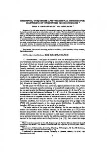
Example

Consider

the

example

2.1

if

A  { x  R : | x1 |  | x2 | 1}  MCC( R ) . It is obvious n

X (t )  { x  R2 :| x1 |  | x2 | et

t

  h( F (t , s, X ( s)), F (t , s, Y ( s))) ds

3.1.

2

is the solution (see Figure 3.1).

0 t

 L  h( X ( s), Y ( s))ds  L t  L d 0

Similarly, t

h( X (t ), Y (t ))  L  L s ds  0

h( X (t ), Y (t )) 

L2 t 2 L2 d 2  ,..., 2! 2!

Lk  d k k!

Then   max h( X (t ), Y (t ))  t[0, d ]

Lk  d k k!

. Therefore,

Lk d k Lk d k for any k  N that contradicts lim 0. k! k  k ! This concludes the proof. 1

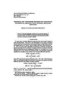
Finally we consider example for case CC ( R2 ) . Example 3.1. Consider the following set-valued integral equation t

1 X (t )   X ( s)ds  S1    0 0

(2.4)

Figure 3.1. The graph of a solution of example 3.1

References [1] [2] [3]

where X () : R  CC( R ) . It is obvious that 1

2

 e t  X (t )  S t   e  0    is the solution of equation (2.4) (see Figure 2.1)

[4] [5] [6] [7] [8] [9]

[10] [11] Figure 2.1. The graph of a solution of system (2.4)

3. Conclusion Also it is possible to prove the similar results if instead

[12] [13] [14]

n

of CC ( R ) we consider a space of all nonempty M strongly convex closed sets of R n and all elements of R n [29], i.e. MCC ( Rn ) .

[15]

de Blasi, F.S., Iervolino, F., “Equazioni differentiali con soluzioni a valore compatto convesso.” Boll. Unione Mat. Ital. 2 (4-5). 491501. 1969. Drici, Z., Mcrae, F.A., Vasundhara Devi, J., “Set differential equations with causal operators.” Math. Probl. Eng. 2. 185-194. 2005. Galanis, G.N., Gnana Bhaskar, T., Lakshmikantham, V., Palamides, P.K., “Set value functions in Frechet spaces: Continuity, Hukuhara differentiability and applications to set differential equations.” Nonlinear Anal., Theory Methods Appl., Ser. A, Theory Methods, 61. 559-575. 2005. Galanis, G.N., Tenali, G.B., Lakshmikantham, V., “Set differential equations in Frechet spaces.” J. Appl. Anal. 14. 103-113. 2008. Lakshmikantham, V., “Set differential equations versus fuzzy differential equations.” Appl. Math. Comput. 164. 277-294. 2005. Lakshmikantham, V., Granna Bhaskar, T., Vasundhara Devi, J., Theory of set differential equations in metric spaces. Cambridge Scientific Publishers, 2006. Laksmikantham, V., Leela, S., Vatsala, A.S., “Interconnection between set and fuzzy differential equations.” Nonlinear Anal., Theory Methods Appl., Ser. A, Theory Methods. 54. 351-360. 2003. Lakshmikantham, V., Mohapatra, R.N., Theory of fuzzy differential equations and inclusions. London, Taylor & Francis, 2003. Perestyuk, N.A., Plotnikov, V.A., Samoilenko, A.M., Skripnik, N.V., Differential equations with impulse effects: multivalued right-hand sides with discontinuities. de Gruyter Stud. Math.: 40, Berlin/Boston: Walter De Gruyter GmbH\& Co., 2011. Piszczek, M., “On a multivalued second order differential problem with Hukuhara derivative.” Opuscula Math. 28 (2). 151-161. 2008. Plotnikov, A.V., Skripnik, N.V., Differential equations with ''clear'' and fuzzy multivalued right-hand side. Asymptotics methods. Odessa, AstroPrint, 2009. (in Russian). Plotnikov, V.A., Plotnikov, A.V., Vityuk, A.N., Differential equations with multivalued right-hand side. Asymptotic methods. Odessa, AstroPrint, 1999. (in Russian). Plotnikova, N.V., “Approximation of a pencil of solutions of linear differential inclusions.” Nonlinear Oscil. (N. Y.). 9 (3). 375390. 2006. Tolstonogov, A., Differential inclusions in a Banach space. Dordrecht, Kluwer Academic Publishers, 2000. Plotnikov, A.V., Tumbrukaki, A.V., “Integro-differential equations with multivalued solutions.” Ukr. Math. J. 52(3). 413423. 2000.

American Journal of Applied Mathematics and Statistics [16] Ahmad, B., Sivasundaram,, S., “ 0 -stability of impulsive hybrid [17] [18] [19] [20] [21] [22]

setvalued differential equations with delay by perturbing lyapunov functions.” Commun. Appl. Anal. 12 (2). 137-146. 2008. Arsirii, A.V., Plotnikov, A.V., “Systems of control over set-valued trajectories with terminal quality criterion.” Ukr. Math. J. 61 (8). 1349-1356. 2009. Plotnikov, A.V., Arsirii, A.V., “Piecewise constant control set systems.” American Journal of Computational and Applied Mathematics. 1 (2). 89-92. 2011. Plotnikov, V.A., Kichmarenko, O.D., “Averaging of controlled equations with the Hukuhara derivative.” Nonlinear Oscil. (N. Y.). 9(3). 365-374. 2006. Plotnikov, A.V., Skripnik, N.V., “Existence and Uniqueness Theorem for Set Integral Equations.” J. Adv. Res. Dyn. Control Syst. 5 (2). 65-72. 2013. Tise, I., “Set integral equations in metric spaces.” Math. Morav. 13 (1). 95-102. 2009. Plotnikov, A.V., “Averaging differential embeddings with Hukuhara derivative.” Ukr. Math. J. 41 (1). 112-115. 1989.

45

[23] Balachandran, K., Prakash, P., “On fuzzy Volterra integral [24] [25] [26] [27] [28] [29]

equations with deviating arguments.” Journal of Applied Mathematics and Stochastic Analysis. 2004 (2). 169-176. 2004. Friedman, M., Ming, M., Kandel, A., “Numerical solution of fuzzy differential and integral equations.” Fuzzy Sets and System. 106. 35-48. 1999. Wang, H., Liu, Y., “Existence results for fuzzy integral equations of fractional order.” Int. Journal of Math. Analysis. 5 (17). 811818. 2011. Rådström, H., “An embedding theorem for spaces of convex sets.” Proc. Amer. Math. Soc. 3. 165-169. 1952. Hukuhara, M., “Integration des applications mesurables dont la valeur est un compact convexe.” Funkcial. Ekvac. 10. 205-223. 1967. Polovinkin, E.S., “Strongly convex analysis.” Sb. Math. 187. 259286. 1996. Balashov, M.V., Polovinkin, E.S., “M-strongly convex subsets and their generating sets.” Sb. Math. 191. 25-60. 2000.