Jul 30, 2016 - This may be viewed as a natural bridge between combinatorics, .... vided that the sizes of the structures in the sequence tend to infinity.
EXISTENCE OF MODELING LIMITS FOR SEQUENCES OF SPARSE STRUCTURES
arXiv:1608.00146v1 [math.CO] 30 Jul 2016
ˇ ˇ JAROSLAV NESET RIL AND PATRICE OSSONA DE MENDEZ
Abstract. A sequence of graphs is FO-convergent if the probability of satisfaction of every first-order formula converges. A graph modeling is a graph, whose domain is a standard probability space, with the property that every definable set is Borel. It was known that FO-convergent sequence of graphs do not always admit a modeling limit, and it was conjectured that this is the case if the graphs in the sequence are sufficiently sparse. Precisely, two conjectures were proposed: (1) If a FO-convergent sequence of graphs is residual, that is if for every integer d the maximum relative size of a ball of radius d in the graphs of the sequence tends to zero, then the sequence has a modeling limit. (2) A monotone class of graphs C has the property that every FO-convergent sequence of graphs from C has a modeling limit if and only if C is nowhere dense, that is if and only if for each integer p there is N (p) such that no graph in C contains the pth subdivision of a complete graph on N (p) vertices as a subgraph. In this paper we prove both conjectures. This solves some of the main problems in the area and among others provides an analytic characterization of the nowhere dense–somewhere dense dichotomy.
1. Introduction Combinatorics is at a crossroads of several mathematical fields, including logic, algebra, probability, and analysis. Bridges have been built between these fields (notably at the instigation of Leibniz and Hilbert). From the interactions of algebra and logic is born model theory, which is founded on the duality of semantical and syntactical elements of a language. Several frameworks have been proposed to unify probability and logic, which mainly belong to two kinds: probabilities over models (Carnap, Gaifman, Scott and Kraus, Nilsson, V¨a¨an¨anen, Valiant,. . . ), and models with probabilities (H. Friedman, Keisler and Hoover, Terwijn, Goldbring and Towsner,. . . ). See [19] for a partial overview. Recently, new bridges appeared between combinatorics and analysis, which are based on the concept of graph limits (see [21] for an in-depth exposition). Two main directions were proposed for the study of a “continuous limit” of finite graphs by means of statistics convergence: • the left convergence of a sequence of (dense) graphs, for which the limit object can be either described as an infinite exchangeable random graph Date: August 2, 2016. Supported by grant ERCCZ LL-1201 and CE-ITI P202/12/G061, and by the European Associated Laboratory “Structures in Combinatorics” (LEA STRUCO). Supported by grant ERCCZ LL-1201 and by the European Associated Laboratory “Structures in Combinatorics” (LEA STRUCO). 1
2
ˇ ˇ JAROSLAV NESET RIL AND PATRICE OSSONA DE MENDEZ
(that is a probability measure on the space of graphs over N that is invariant under the natural action of Sω ) [2, 16], or as a graphon (that is a measurable function W : [0, 1] × [0, 1] → [0, 1]) [6, 7, 22]. • the local convergence of a sequence of bounded degree graphs, for which the limit object can be either described as a unimodular distribution (a probability distribution on the space of rooted connected countable graphs with bounded degrees satisfying some invariance property) [3], or as a graphing (a Borel graph that satisfies some Intrinsic Mass Transport Principle or, equivalently, a graph on a Borel space that is defined by means of finitely many measure preserving involutions) [9]. A general (unifying) framework has been introduced by the authors, under the generic name “structural limits” [29]. In this setting, a sequence of structures is convergent if the satisfaction probability of every formula (in a fixed fragment of first-order logic) for a (uniform independent) random assignment of vertices to the free variables converges. The limit object can be described as a probability measure on a Stone space invariant by some group action, thus generalizing approaches of [2, 16] and [3]. This may be viewed as a natural bridge between combinatorics, model theory, probability theory, and functional analysis [33]. The existence of a graphing-like limit object, called modeling, has been studied in [31, 35], and the authors conjectured that such a limit object exists if and only if the structures in the sequence are sufficiently “structurally sparse”. For instance, the authors conjectured that if a convergent sequence is non-dispersive (meaning that the structures in the sequence have no “accumulation elements”) then a modeling limit exists: Conjecture 1 ([35]). Every convergent residual sequence of finite structures admits a modeling limit. For the case of sequences of graphs from a monotone class (that is a class of finite graphs closed by taking subgraphs) the authors conjectured the following exact characterization, where nowhere dense classes [27, 28] form a large variety of classes of sparse graphs, including all classes with excluded minors (as planar graphs), bounded degree graphs and graph classes of bounded expansion [24, 25, 26]. Conjecture 2 ([31]). A monotone class of graphs C admits modeling limits if and only if C is nowhere dense. Note that this conjecture is known in one direction [31]. To prove the existence of modeling limits for sequences of graphs in a nowhere dense class is the main problem addressed in this paper. Nowhere dense classes enjoy a number of (non obviously) equivalent characterizations and strong algorithmic and structural properties [30]. For instance, deciding properties of graphs definable in first-order logic is fixed-parameter tractable on nowhere dense graph classes (which is optimal when the considered class is monotone, under a reasonable complexity theoretic assumption) [15]. Modeling limits exist for sequences of graphs with bounded degrees (as graphings are modelings), and this has been so far verified for sequences of graphs with bounded tree-depth [31], for sequences of trees [35], for sequences of plane trees and sequences of graphs
EXISTENCE OF MODELING LIMITS FOR SEQUENCES OF SPARSE STRUCTURES
3
with bounded pathwidth [14], and for sequences of mappings [34] (which is the simplest form of non relational nowhere dense structures). (See also related result on sequences of matroids [17].) In this paper, we prove both Conjecture 1 and Conjecture 2 in their full generality. Our paper is organized as follows: In Section 2 we recall all necessary notions, definitions, and notations. In Section 3 we will deal with limits with respect to the fragment FO1 of all first-order formulas with at most one free variable. In Section 5 we deduce a proof of Conjecture 1 and, using a characterization of nowhere denses from [36], we prove that Conjecture 2 holds. Finally, we discuss some possible developments in Section 6. The general proof strategy is depicted bellow:
Friedman L(Qm ) logic
Structural Limits
Nowhere dense classes
Modeling FO1 -limits
Lift of nowhere dense sequences
Modeling limits of �-residual sequences
Countable skeleton
Modeling limits for nowhere dense classes
2. Preliminaries, Definitions, and Notations 2.1. Structures and Formulas. A signature is a set σ of function or relation symbols, each with a finite arity. In this paper we consider finite or countable signatures. A σ-structure A is defined by its domain A, and by the interpretation of the symbols in σ, either as a relation RA (for a relation symbol A) or as a function f A (for a function symbol f ). A signature σ also defines the (countable) set FO(σ) of all first-order formulas built using the relation and function symbols in σ, equality, the standard logical conjunctives, and quantification over elements of the domain. The quotient of FO(σ) by logical equivalence has a natural structure of countable Boolean algebra, the Lindenbaum-Tarski algebra B(FO(σ)) of FO(σ). For a formula φ with p free variables and a structure A we denote by φ(A) the set of all satisfying assignments of φ in A, that is φ(A) = {(v1 , . . . , vp ) ∈ Ap : A |= φ(v1 , . . . , vp )}. If A is a finite structure (or a structure whose domain is a probability space), we define the Stone pairing hφ, Ai of φ and A as the probability of satisfaction of φ in A for a random assignments of the free variables. Hence if A is finite (and no
4
ˇ ˇ JAROSLAV NESET RIL AND PATRICE OSSONA DE MENDEZ
specific probability measure is specified on the domain of A) it holds hφ, Ai =
|φ(A)| . |A|p
Generally, if the domain of A is a probability space (with probability measure νA ) and φ(A) is measurable then ⊗p hφ, Ai = νA (φ(A)), ⊗p where νA denotes the product measure on Ap . For a σ-structure A we denote by Gaifman(A) the graph with vertex set A, such that two (distinct) vertices x and y are adjacent in Gaifman(A) if both belong to some relation in A (that is if ∃R ∈ σ : {x, y} ⊆ RA ).
2.2. Stone Space and Representation by Probability Measures. The term of Stone pairing comes from a functional analysis point of view: Let S(FO(σ)) be the Stone dual of the Boolean algebra B(FO(σ)). Points of S(FO(σ)) are equivalently described as the ultrafilters on B(FO(σ)), the homomorphisms from B(FO(σ)) to the two-element Boolean algebra, or the maximal consistent sets T of formulas from FO(σ) (point of view we shall make use of here). The space S(FO(σ)) is a compact totally disconnected Polish space, whose topology is generated by its clopen sets k(φ) = {T ∈ S(FO(σ)) : φ ∈ T }. Let A be a finite σ-structure (or a σ-structure on a probability space such that every first-order definable set is measurable). Identifying φ with the indicator function 1k(φ) of the clopen set k(φ), the map φ 7→ hφ, Ai uniquely extends to a continuous linear form on the space C(S(FO(σ))). By Riesz representation theorem there exists a unique probability measure µA such that for every φ ∈ FO(σ) it holds Z hφ, Ai = 1k(φ) dµA . S(FO(σ))
Note that the permutation group Sω defines a (subgroup of the) group of automorphisms of B(FO)(σ) (by permuting free variables) and acts naturally on S(FO(σ)). The probability measure µA associated to the structure A is obviously invariant under the Sω -action. For more details on this representation theorem we refer the reader to [29]. 2.3. Structural Limits. Let σ be a signature, and let X be a fragment of FO(σ). A sequence A = (An )n∈N of σ-structures is X-convergent if hφ, An i converges as n grows to infinity or, equivalently, if the associated probability measures µAn on S(X) converge weakly [29]. In our setting, the strongest notion of convergence is FO-convergence (corresponding to the full fragment of all first-order formulas). Convergence with respect to the fragment QF− (of all quantifier-free formulas without equality) is equivalent to the left convergence introduced by Lov´asz et al [4, 6, 22]. (It is also equivalent to convergence with respect to the fragment QF of all quantifier-free formulas, provided that the sizes of the structures in the sequence tend to infinity.) For bounded degree graphs, convergence with respect to the fragment FOlocal of local formu1 las with a single free variable is equivalent to the local convergence introduced by Benjamini and Schramm [3]. (Recall that a formula is local if its satisfaction only depends on a fixed neighborhood of its free variables.) Also, in this case, local
EXISTENCE OF MODELING LIMITS FOR SEQUENCES OF SPARSE STRUCTURES
5
convergence is equivalent to convergence with respect to the fragment FOlocal of all local formulas, provided that the sizes of the structures in the sequence tend to infinity. For a discussion on the different notions of convergence arising from different choices of the considered fragment of first-order logic, we refer the interested reader to [29, 31, 35]. Note that the equivalence of X-convergence with the weak convergence of the probability measures on S(X) associated to the finite structures in the sequence is stated in [29] as a representation theorem, which generalizes both the representation of the left limit of a sequence of graphs by an infinite random exchangeable graph [2] and the representation of the local limit of a sequence of graphs with bounded degree by an unimodular distribution on the space of rooted connected countable graphs [3]. 2.4. Non-standard Limit Structures. A construction of a non-standard limit object for FO-convergent sequences has been proposed in [29], which closely follows Elek and Szegedy construction for left limits of hypergraphs [10]. One proceeds as follows: Let (An )n∈N be a sequence of finite σ-structures and let U be a non-principal e=Q e ultrafilter. Let A i∈N Ai and let ∼ be the equivalence relation on A defined by (xn ) ∼ (yn ) if {n : xn = yn } ∈ U . Then the ultraproduct of the structures An Q e by ∼, and such is the structure L = U Ai , whose domain L is the quotient of A that for each relational symbol R it holds is defined by ([v 1 ], . . . , [v p ]) ∈ RL
⇐⇒
{n : (vn1 , . . . , vnp ) ∈ RAn } ∈ U.
1 p Q As proved by Lo´s [20], for each formula φ(x1 , . . . , xp ) and each v , . . . , v ∈ n An we have Y Ai |= φ([v 1 ], . . . , [v p ]) iff {i : Ai |= φ(vi1 , . . . , vip )} ∈ U. U
In [29] a probability measure ν is constructed from the normalised counting measures νi of Ai via the Loeb measure construction, and it is proved that every first-order definable set of the ultraproduct is measurable. The ultraproduct is then a limit object for the sequence (An )n∈N . In particular, for every first-order formula φ with p free variables it holds: hφ,
Y U
Z Ai i =
Z ···
1φ ([x1 ], . . . , [xp ]) dν([x1 ]) . . . dν([xp ]) = limhφ, Ai i. U
Moreover, the above integral is invariant by any permutation on the order of the integrations. However, the constructed object is difficult to handle. In particular, the sigmaQ algebra constructed on U An is not separable. For a discussion we refer the reader to [8, 10]. The ultraproduct construction is used in the proof of Lemma 2 to prove consistency of some theories in Friedman’s Qm logic (see Section 2.6). 2.5. Modelings. By similarity with graphings, which are limit objects for local convergent sequences of graphs with bounded degrees [9], the authors proposed the term of modeling for a structure A built on a standard Borel space A, endowed with a probability measure νA , and such that every first-order definable set is Borel [31]. Such structures naturally avoid pathological behaviours (for instance, every
6
ˇ ˇ JAROSLAV NESET RIL AND PATRICE OSSONA DE MENDEZ
definable set is either finite, countable, or has the cardinality of continuum). The definition of Stone pairing obviously extends to modeling by setting (1)
hφ, Ai = ν ⊗p (φ(A)).
An X-convergent sequence (An )n∈N has modeling X-limit L (or simply modeling limit L when X = FO) if L is a modeling such that for every φ ∈ X it holds hφ, Li = lim hφ, An i. n→∞
Let C be a class of structures. We say that C admits modeling limits if every FO-convergent sequence of structures (An )n∈N with An ∈ C has a modeling limit. Note that not every FO-convergent sequence has a modeling limit: Consider a sequence (Gn )n∈N of graphs, where Gn is a graph of order n, with edges drawn randomly (independently) with edge probability 0 < p < 1. Then with probability 1 the sequence (Gn )n∈N is FO-convergent. However, this sequence has no modeling limit, and even no modeling QF− -limit: Assume for contradiction that (Gn )n∈N has a modeling QF-limit L. Because hx1 = x2 , Gn i = 1/n → 0 the probability measure νL is atomless thus L is uncountable. As L is a standard Borel space, there exists zero-measure sets N ⊂ L and N 0 ⊂ [0, 1], and a bijective measure preserving map f : L\N → [0, 1]\N 0 . By the equivalence of QF− -convergence and left-convergence the modeling L defines a {0, 1}-valued graphon W : [0, 1] × [0, 1] → [0, 1], which is a left limit of (Gn )n∈N by: ( 1 if x, y ∈ / N 0 and L |= f −1 (x) ∼ f −1 (y) W (x, y) = 0 otherwise. But a left limit of (Gn )n∈N is the constant graphon p, which is not weakly equivalent to W (as it should, according to [5]) thus we are led to a contradiction. This example is prototypal, and this allows us to prove that if a monotone class of graphs admits modeling limits then this class has to be nowhere dense [31]. The proof involves the characterization of nowhere dense classes by the model theoretical notions of stability and independence property [1], their relation to VC-dimension [18], and the characterization of sequences of graphs admitting a random-free (i.e. almost everywhere {0, 1}-valued) left limit graphon [23]. Conjecture 2 asserts that the converse is true as well. 2.6. H. Friedman’s Qm -logic. Friedman [11, 12] studied a logical system where the language is enriched by the quantifier “there exists x in a non zero-measure set . . . ”, for which he studied axiomatizations, completeness, decidability, etc. A survey including all these results was written by Steinhorn [37, 38]. In particular, H. Friedman considered specific type of models, which he calls totally Borel, which are (almost) equivalent to our notion of modeling: A totally Borel structure is a structure whose domain is a standard Borel space (endowed with implicit Borel measure) with the property that every first-order definable set (with parameters) is measurable. In this context, Friedman introduced a new quantifier Qm , which is to be understood as expressing “there exists non-measure 0 many”, and initiated the study of the extension L(Qm ) of first order logic, whose axioms are all the usual axiom schema for first-order logic together with the following ones [38]: M0 ¬(Qm x)(x = y);
EXISTENCE OF MODELING LIMITS FOR SEQUENCES OF SPARSE STRUCTURES
7
M1 (Qm x)Ψ(x, . . . ) ↔ (Qm y)Ψ(y, . . . ), where Ψ(x, . . . ) is an L(Qm )-formula in which y does not occur and Ψ(y, . . . ) is the result of replacing each free occurrence of x by y; M2 (Qm x)(Φ ∨ Ψ) → (Qm x)Φ ∨ (Qm x)Ψ; M3 [(Qm x)Φ ∧ (∀x)(Φ → Ψ)] → (Qm x)Ψ; M4 (Qm x)(Qm y)Φ → (Qm y)(Qm x)Φ. The rules of inference for L(Qm ) are the same as for first-order logic: modus ponens and generalization. Let the proof system just described be denoted by Km . The standard semantic for Qm is as follows: for a structure M on a probability space such that every first-order definable (with parameters) is measurable (for probability measure λ) it holds M |= Qm x φ(x, a)
⇐⇒
λ({x : M |= φ(x, a)}) > 0.
Note that the set of L(Qm )-sentences satisfied by M (for this semantic) is obviously consistent in Km . The following completeness theorem has been proved by Friedman [11] (see also [38]): Theorem 1. A set of sentences T in L(Qm ) has a totally Borel model if and only if T is consistent in Km . It has been noted that one can require the domain of the totally Borel model to be a Borel subset of R with Lebesgue measure 1. 3. Modeling FO1 -limits Let A = (An )n∈N be an FO-convergent sequence of finite structures, and let A) be the union of a complete theory of an elementary limit of A together with, T (A for each first order formula φ with free variables x1 , . . . , xp , either or
(Qm x1 ) . . . (Qm xp ) φ, � ¬ (Qm x1 ) . . . (Qm xp ) φ ,
if lim hφ, An i > 0; n→∞
if lim hφ, An i = 0. n→∞
A): The ultraproduct construction provides a model for T (A Lemma 2. For every FO-convergent sequence A of finite structures, the theory A) is consistent in Km . T (A Proof. Using the standard semantic for Qm it is immediate that any ultraproduct Q A) hence T (A A) is consistent in Km . A � i is a model for T (A U
Theorem 3. For every FO-convergent sequence A of finite structures, there exists a modeling M whose domain M is a Borel subset of R, and such that: (1) the probability measure νM associated to M is uniformly continuous with respect to Lebesgue measure λ; (2) M is a modeling FO1 -limit of A ; (3) for every φ ∈ FO it holds hφ, Mi = 0
⇐⇒
lim hφ, An i = 0.
n→∞
8
ˇ ˇ JAROSLAV NESET RIL AND PATRICE OSSONA DE MENDEZ
A) is consistent in Km . Hence, accordProof. According to Lemma 2 the theory T (A A) has a totally Borel model T. (Furthermore, we may assume ing to Theorem 1, T (A that T is a Borel subset of R with Lebesgue measure 1.) k For every integer k, there exists an integer N (k) and N (k) formulas θ1k , . . . , θN (k) (with a single free variable) defining the local 1-types up to quantifier rank k in the sense that all of these formulas are local and have W quantifier rank k, they induce a partition (formalized as θik ` ¬θjk if i 6= j and ` i θik ), and for every local formula φ(x) with quantifier rank k and for every 1 ≤ i ≤ N (k) either it holds θik ` φ, or θik ` ¬φ. Define Ik = {i : λ(θik (L)) > 0}. Define the probability measure πk on L as follows: for every Borel subset X of L define X λ(X ∩ θk (L)) i πk (X) = · lim hθik , Gn i. k (L)) n→∞ λ(θ i i∈I k
Obviously πk weakly converges to some probability measure π. Let M be the modeling obtained by endowing L with the probability measure νM = π. Note that νM is absolutely continuous with respect to λ by construction. � Theorem 3 immediately implies Corollary 1. Every FO1 -convergent sequence has a modeling FO1 -limit.
4. Modeling Limits of Residual Sequences We know that in general an FO-convergent sequence does not have a modeling limit (hence Corollary 1 does not extend to full FO). This nicely relates to sparse– dense dichotomy. Recall that a class C of (finite) graphs is nowhere dense if, for every integer k, there exists an integer n(k) such that the k-th subdivision of the complete graph Kn(k) on n(k) vertices is the subgraph of no graph in C [27, 30]. (Note a subgraph needs not to be induced.) Based on a characterization by Lov´asz and Szegedy [23] or random-free graphon and a characterization of nowhere-dense classes in terms of VC-dimension (Adler and Adler [1] and Laskowski [18]) the authors derived in [31] the following necessary condition for a monotone class C to have modeling limits. Theorem 4. Let C be a monotone class of graphs. If every FO-convergent of graphs from C has a modeling limit then the class C is nowhere dense. However, there is a particular case where a modeling limit for an FO-convergent sequence will easily follow from Theorem 3. That will be done next. Definition 5. A sequence (An )n∈N is residual if, for every integer d it holds lim
sup
n→∞ vn ∈An
|Bd (An , vn )| = 0, |An |
where Bd (An , vn ) denotes the set of elements of An at distance at most d from vn (in the Gaifman graph of An ). Equivalently, (An )n∈N is residual if, for every integer d, it holds lim hdist(x1 , x2 ) ≤ d, An i = 0. n→∞
EXISTENCE OF MODELING LIMITS FOR SEQUENCES OF SPARSE STRUCTURES
9
The notion of residual sequence is linked to the one of residual modeling: A residual modeling is a modeling, all components of which have zero measure (that is if and only if for every integer d, every ball of radius d has zero measure). By an interplay of these notions we now can prove Conjecture 1. Theorem 6. Every FO-convergent residual sequence has a modeling limit.
Proof. The main characteristic of residual sequences is that a residual sequence is FO-convergent if and only if it is FO1 -convergent [35]. Consider the modeling limit M obtained in Theorem 3 for a FO-convergent residual sequence. Then for every integer d it holds hdist(x1 , x2 ) ≤ d, Mi = 0. It follows that M is residual, and thus the convergence of hφ, An i to hφ, Mi for first-order formulas with (at most) one free variable (i.e. FO1 -convergence) implies convergence for all first-order formulas (i.e. FO-convergence). � 5. Modeling Limits of Quasi-Residual Sequences Here we prove our main result in the form of a generalization of Section 4 for quasi-residual sequences. The motivation for the introduction of the definition of quasi-residual sequences is the following: Known constructions of modeling limits for some nowhere dense classes with unbounded degrees [14, 31, 35] are based on the construction of a countable “skeleton” on which residual parts are grafted. We shall use the same idea here for the general case. The countable skeleton will be built thanks to the following characterization of nowhere dense classes proved in [36]: Theorem 7. Let C be a class of graphs. Then C is nowhere dense if and only if for every integer d and every � > 0 there is an integer N = N (d, �) with the following property: for every graph G ∈ C, and every subset A of vertices of G, there is S ⊆ A with |S| ≤ N such that no ball of radius d in G[A \ S] has order greater than � |A|. This theorem justifies the introduction of the following relaxation of the notion of residual sequence: Definition 8. A sequence (An )n∈N (with |An | → ∞) is quasi-residual if, for every integer d and every � > 0 there exists an integer N such that it holds lim sup
inf
sup
n→∞ Sn ∈(ANn ) vn ∈An \Sn
|Bd (Gaifman(An ) \ Sn , vn )| < �. |An |
In other words, (An )n∈N is quasi-residual if, for every distance d and every � > 0 there exists an integer N so that (for sufficiently large n) one can remove at most N vertices in the Gaifman graph of An so that no ball of radius d will contain at least � proportion of An . The next result directly follows from Theorem 7. Corollary 2. Let C be a nowhere dense class of graphs and let (Gn )n∈N be a sequences of graphs from C such that |Gn | → ∞. Then (Gn )n∈N is quasi-residual.
ˇ ˇ JAROSLAV NESET RIL AND PATRICE OSSONA DE MENDEZ
10
5.1. (d, �)-residual Sequences. We now consider a relaxation of the notion of residual sequence and show how this allows to partially reduce the problem of finding modeling FO-limits to finding modeling FO1 -limits. Definition 9. Let d be an integer and let � be a positive real. A sequence (An )n∈N is (d, �)-residual if it holds lim sup sup n→∞
vn ∈An
|Bd (An , vn )| < �. |An |
Similarly, a modeling M is (d, �)-residual if it holds sup νM (Bd (M, v)) < �. v∈M
Lemma 10. Let d ∈ N and let � > 0 be a positive real. Assume (An )n∈N is a FOconvergent (2d, �)-residual sequence of graphs and assume L is a (2d, �)-residual modeling FO1 -limit of (An )n∈N . Then for every d-local formula φ with p free variables it holds |hφ, Li − lim hφ, An i| < p2 �. n→∞
Proof. By restricting the signature to the symbols in φ if necessary, we can assume that σ is finite. Let q be the quantifier rank of φ. Then there exists finitely many local formula ξ1 , . . . , ξN with quantifier rank at most q (expressing the rank q d-local type) such that: W • every element of every model satisfies exactly one of the ξi (formally, ` ξi and ` (ξi → ¬ξj ) if i 6= j); • two elements x and y satisfies the same local first-order formulas of quantifier rank at most q if and only if they satisfy the same ξi . V Let ζ(x1 , . . . , xp ) be the formula 1≤i2d (xi , xj ). By d-locality of φ there exists a subset X ⊆ [N ]p such that p h i _ ^ ζ` φ↔ ξij (xj ) . (i1 ,...,ip )∈X j=1
Let φe =
W
(i1 ,...,ip )∈X
Vp
j=1 ξij (xj ).
e Ai = hφ,
For every structure A it holds X
p Y
hξij , Ai.
(i1 ,...,ip )∈X j=1
As L is a modeling FO1 -limit of An it holds hξij , Li = limn→∞ hξij , An i, hence e Li = lim hφ, e An i. hφ, n→∞
e for every structure A holds On the other hand, as ζ ` (φ ↔ φ), � � e Ai| ≤ h¬ζ, Ai ≤ p hd≤2d , Ai. |hφ, Ai − hφ, 2 Note that hd≤2d , Ai is nothing but the expected measure of a ball of radius 2d in e Ai| < �. Thus, A. In particular, if A is (2d, �)-residual, then it holds |hφ, Ai − hφ, |hφ, Li − lim hφ, An i| < p2 �. n→∞
�
EXISTENCE OF MODELING LIMITS FOR SEQUENCES OF SPARSE STRUCTURES
11
5.2. Marked Quasi-residual sequences. To allow an effective use of the properties of quasi-residual sequences, we use a (lifted) variant of the notion of quasiresidual sequence. Let σ be a countable signature and let σ + be the signature obtained by adding to σ countably many unary symbols {Mi }i∈N and {Zi }i∈N . For integers d, i we define the formulas δd,i and δˆd as (2)
δd,i := (∃z) d≤d (x1 , z) ∧ Mi (z)
(3)
δˆd := (∃z) d≤d (x1 , z) ∧ Zd (z)
In other words, δd,i (x) holds if x belongs to the ball of radius d centered at the element marked Mi , and δˆd (x) holds if x belongs to the d-neighborhood of elements marked by Zd . + + Definition 11. A sequence (A+ n )n∈N (with |An | → ∞) of σ -structures is a marked quasi-residual sequence if the following condition holds:
• For every integers i, n it holds |Mi (A+ n )| ≤ 1 (i.e. at most one element in is marked by M ); A+ i n • For every distinct integers i, j and every integer n, no element of A+ n is marked both Mi and Mj ; • For every integer d there is a non-decreasing unbounded function Fd : N → N with the property that for every integer n it holds Fd (n)
Zd (A+ n) =
(4)
[
Mi (A+ n );
i=1
(5)
• For every integer d and every positive real � > 0 there is N ∈ N such that SN + |Bd (Gaifman(A+ n) \ i=1 Mi (An ), vn )| lim sup sup < �. + SN + |An | n→∞ vn ∈A+ n \ i=1 Mi (An ) SN + (In other words, every ball of radius d in Gaifman(A+ n) \ i=1 Mi (An ) contains less than � proportion of all the vertices, as soon as n is sufficiently large.) • For every integer d the following limit equality holds:
(6)
lim hδˆd , A+ n i = lim lim h
n→∞
m→∞ n→∞
m ^
δd,m , A+ n i.
i=1
The main purpose of this admittedly technical definition is to allow to make use of the sets Sn arising in the definition of quasi-residual sequences by first-order formula, by means of the marks Mi . The role of the marks Zd is to allow a kind of of limit exchange. (Note that δd,i (A+ ) is nothing but the ball of radius d of A+ centered at the element marked by Mi .) Lemma 12. For every quasi-residual sequence (An )n∈N of σ-structures there exists an FO-convergent marked quasi-residual sequence (B+ n )n∈N of σ-structures such that (Forget(B+ )) is a subsequence of (A ) . n n∈N n n∈N Proof. Let σ 0 be the signature obtained by adding to σ countably many unary symbols {Mi }i∈N . For n ∈ N we define the σ 0 -structure A0n has the σ 0 -structure
ˇ ˇ JAROSLAV NESET RIL AND PATRICE OSSONA DE MENDEZ
12
obtained from An by defining marks Mi are assigned in such a way that for every SN d ∈ N and � > 0 there is N ∈ N such that letting Sn = i=1 Mi (A0n ) it holds lim sup
sup
n→∞
vn ∈A0n \Sn
|Bd (Gaifman(A0n ) \ Sn , vn )| < �. |A0n |
This is obviously possible, thanks to the definition of a quasi-residual sequence. Considering an FO-convergent subsequence we may assume that (A0n ) is FOconvergent. For d ∈ N we define the constant m _ αd = lim lim h δd,i , A0n i. m→∞ n→∞
i=1
Wm (Note that the values limn→∞ h i=1 δd,i , A0n i exist as (A0n ) is FO-convergent and that they form, for increasing m, a non-decreasing sequence bounded by 1.) Then for each d ∈ N there exists a non-decreasing function Fd : N → N such that limn→∞ lim Fd (n) = ∞ and F (n)
lim h
n→∞
define A+ to be the SFd (n)n in i=1 Mi (A0n ).
Then we elements (A+ n )n∈N .
_
δd,i , A0n i = αd .
i=1
sequence obtained from A0n by marking by Zd all the Now we let (B+ n ) to be a converging subsequence of �
Let ζd be the formula asserting that the ball of radius d centered at x1 contains x2 but no element marked Zd , that is ζd := d≤d (x1 , x2 ) ∧ (∀z)(d≤d (x1 , z) → ¬Zd (z)). Lemma 13. Let (A+ n )n∈N be a marked quasi-residual sequence. Then lim hζd , A+ n i = 0.
n→∞
Proof. Assume for contradiction that a = limn→∞ hζd , A+ n i is strictly positive. According to the definition of a marked quasi-residual sequence, there exists an Sm integer m such that no ball of radius d in Gaifman(A+ M (A+ i n) \ n ) contains i=1 more than (a/2)|An | elements. Let n0 be such that Fd (n0 ) ≥ m, and let n1 ≥ n0 be such that hζd , A+ n i > a/2 holds for every n ≥ n1 . Then there exists v such that the ball of radius d centered at v contains no element marked Zd (hence no element marked M1 , . . . , Mm ) and contains more than (a/2)|An | elements, the fact that this ball is a ball of radius Sm what contradicts + d in Gaifman(A+ � n) \ i=1 Mi (An ). In general, a modeling FO1 -limit of a (d, �)-residual sequence does not need to be (d0 , �0 )-residual. However, if we consider a sequence that is also marked quasiresidual, and if we assume that the modeling FO1 -limit satisfies the additional properties asserted by Theorem 3 then we can conclude that the modeling is (d/4, �)residual, as proved in the next lemma. + Lemma 14. If the sequence (A+ n ) is (4d, �)-residual and L is a modeling with the + properties asserted by Theorem 3 then L is (d, �)-residual.
EXISTENCE OF MODELING LIMITS FOR SEQUENCES OF SPARSE STRUCTURES
13
Proof. We first prove that the set Υ of vertices v ∈ L+ such that the ball of radius 2d centered at v has measure greater than � has zero measure. According to + Lemma 13, it holds limn→∞ hζ2d , A+ n i = 0 hence hζ2d , L i = 0. This implies that the set V of x1 such that the ball of radius 2d centered at x1 contains no element marked Z2d and has measure at least � has zero measure. Hence we only have to consider vertices v in the 2d-neighborhood of Z2d (L+ ). Let α2d = lim lim h m→∞ n→∞
m _
δ2d,i , An +i.
i=1
Let k ∈ N. There exists m(k) such that m(k)
(7)
lim h
n→∞
_
δ2d,i , A+ n i > α2d − 1/k,
i=1
which means that at least α2d − 1/k proportion of L+ is at distance at most 2d from elements marked M1 , . . . , Mm(k) . However, according to (6), and as L+ is a modeling FO1 -limit of (A+ n )n∈N it holds + ˆ α2d = lim hδˆ2d , A+ n i = hδ2d , L i, n→∞
which means that a α2d proportion of L+ is at distance at most 2d from elements marked Z2d (which include elements marked M1 , . . . , Mm(k) ). Thus the set Nk of vertices in the 2d-neighborhood of Z2d (L+ ) but not in the 2d-neighborhood of Sm(k) + i=1 Mi (L ) has measure at most 1/k. Sm(k) Let v be in the 2d-neighborhood of i=1 Mi (L+ ). Then the ball of radius 2d centered at v is included in the ball of radius 4d centered at a vertex marked Mi , for some i ≤ m(k). But this ball has measure hδ4d,i , L+ i = limn→∞ hδ4d,i , A+ n i. As + i < � for sufficiently large ) is (4d, �)-residual, it holds hδ , A the sequence (A+ 4d,i n n n. Hence the ball of L+ of radius 2d centered at v (which is included in the ball of radius 4d centered at the vertex marked Mi ) has measure less than �. It follows that the set of v such that T the ball of radius 2d centered at v has measure at least � is included in V ∪ k Nk hence has zero measure. Now assume for contradiction that there exists a vertex v such that the ball B of radius d centered at v has measure at least �. Then for every w ∈ B the ball of radius 2d centered at v has measure at least �, what contradicts the fact that the measure of B is positive. � 5.3. Color Coding and Mark Elimination. We now consider how to turn a marked quasi-residual into a (d, �)-residual marked quasi-residual sequence. The idea here, is to encode each relation R with arity k > 1 with mk −1 relations plus a sentence. The sentence expresses the behaviour of R when restricted to elements marked M1 , . . . , Mm . The mk − 1 relations expresses which tuples of nonmarked elements can be extended (and how) with elements marked M1 , . . . , Mm to form a k-tuple of R. As above, let σ + be a countable signature with unary relations Mi and Zi . Let m ∈ N. We define the signature σ ∗m as the signature obtained from σ + by adding, for R of arity k −|I|, where each symbol R ∈ σ with arity k > 1 the relation symbols NI,f ∅= 6 I ( [k] and f : I → [m].
ˇ ˇ JAROSLAV NESET RIL AND PATRICE OSSONA DE MENDEZ
14
Let A+ be a σ + -structure. We define the structure Encodem (A+ ) as the σ ∗m -structure A∗ , which has same domain as A+ , same unary relations, and such that for every symbol R ∈ σ + with arity k > 1, for every ∅ 6= I ( [k] and f : I → [m], denoting i1 < · · · < i` the elements of [k] \ I and i`+1 , . . . , ik the elements of I, it holds R A∗ |= NI,f (vi1 , . . . , vi` )
⇐⇒ A+ |=
` ^ m ^
k h ^ �i ¬Mr (vij ) ∧ (∃vi`+1 , . . . , vik ) R(v1 , . . . , vk ) ∧ Mf (ij ) (vij )
j=1 r=1
j=`+1
and A∗ |= R(v1 , . . . , vk ) +
⇐⇒ A |= R(v1 , . . . , vk ) ∧
k ^ m ^
¬Mj (vi ).
i=1 j=1
Note that the Gaifman graph of A∗ can be obtained from the Gaifman graph of A by removing all edges incident to a vertex marked M1 , . . . , Mm . We now explicit how the relation R in A+ can be retrieved from A∗ . Z,m For m ∈ N, R ∈ σ with arity k > 1, and Z ⊆ [m]k let ηR (x1 , . . . , xk ) be defined as follows: +
Z,m ηR :=
k ^
_
k ^ m h i ^ Mij (xi ) ∨ R(x1 , . . . , xk ) ∧ ¬Mj (xi )
(i1 ,...,ik )∈Z j=1
_ h
_
∨
i=1 j=1
NI,f (xi1 , . . . , xi` ) ∧
^
Mf (i) (xi ) ∧
m ^
¬Mj (xi )
i
i∈[k]\II j=1
i∈I
∅6=I⊆[k] f :I→[m]
^
Z be the following sentence, which expresses that Z encodes the set of and let ςR all the tuples of elements marked M1 , . . . , Mm in R.
Z ςR
:=
h
^
(∃x1 , . . . , xk ) R(x1 , . . . , xk ) ∧
�i (Mij (xi )
j=1
(i1 ,...,ik )∈Z
∧¬
k ^
h
_
k ^
(∃x1 , . . . , xk ) R(x1 , . . . , xk ) ∧
�i (Mij (xi ) .
j=1
(i1 ,...,ik )∈[m]k \Z
The following lemma sums up the main properties of our construction. Lemma 15. Let A+ be a σ + -structure, and let A∗ = Encodem (A+ ). Let R ∈ σ be a relation symbol with arity k > 1. Then Z • there exists a unique subset Z of [m]k such that A+ |= ςR + • for this Z and for every v1 , . . . , vk ∈ A it holds
A+ |= R(v1 , . . . , vk )
⇐⇒
Z,m A∗ |= ηR (v1 , . . . , vk ).
Proof. This lemma straightforwardly follows from the above definitions.
�
EXISTENCE OF MODELING LIMITS FOR SEQUENCES OF SPARSE STRUCTURES
15
Let m ∈ N be fixed. An elimination theory is a set Tm containing, for each R ∈ σ with arity k > Z 1, exactly one sentence ςR (for some Z ⊆ [m]k ). For a σ + -structure A+ , the + Z elimination theory of A is the set of all sentences ςR satisfied by A+ . For a formula φ ∈ FO(σ), we define the elimination formula φb of φ with respect to an elimination theory Tm as the formula obtained from φ by replacing each Z,m occurence of relation symbol R with arity k > 1 by the formula ηR , where Z is Z the unique subset of [m]k such that ςR ∈ Tm . It directly follows from Lemma 15 that if A+ is a σ + -structure which satisfies all sentences in an elimination theory Tm , then for every formula φ ∈ FO(σ), denoting φb the elimination formula of φ with respect to Tm it holds (8)
b 1 , . . . , vp ) Encodem (A+ ) |= φ(v
⇐⇒
A+ |= φ(v1 , . . . , vp ).
5.4. Modeling Limits of Quasi-residual Sequences. Let us recall Gaifman locality theorem. Theorem 16 ([13]). Every first-order formula ψ(x1 , . . . , xn ) is equivalent to a Boolean combination of t-local formulae χ(xi1 , . . . , xis ) and basic local sentences of the form m �^ � ^ ∃y1 . . . ym φ(yi ) ∧ d>2r (yi , yj ) i=1
1≤i 0 be a positive real. Let d = 7q−1 /2 and let m and Smn0 be integers such that for every2 n ≥ n0 no ball of radius 8d in Gaifman(An ) \ i=1 Mi (A+ n ) contains at least (�/p )|An | vertices. Let A∗n = Encodem (A+ ). Each relation of A∗n being defined by a fixed forn + mula from relations of An , the sequence (A∗n )n∈N is FO-convergent and L∗ = Encodem (L+ ) is a modeling FO1 -limit of (A∗n )n∈N satisfying additional properties asserted by Theorem 3. Let Tm be the elimination theory of L+ (as defined above). As L+ is an FO1 limit (hence an elementary limit) of (A+ n )n∈N there exists n1 ≥ n0 such that for Z Z every symbol R ∈ σ with arity k > 1 used in φ, if ςR ∈ Tm then A+ n |= ςR holds for every n ≥ n1 . Let φb be the elimination formula of φ with respect to Tm . Note that φb has also quantifier rank at most q. According to Lemma 15, for every n ≥ n1 it b ∗ ) = φ(A+ ). Thus, as φ(A+ ) = φ(An ) (as φ only uses symbols in σ) it holds φ(A n n n holds (9)
b A∗ i = hφ, An i. hφ, n
∀n ≥ n1
As L∗ satisfies Tm we get b L∗ i = hφ, Li. hφ,
(10)
Note that by our choice of m the sequence (A∗n ) is (8d, �/p2 )-residual hence by Lemma 14 the modeling L∗ is (2d, �/p2 )-residual. According to Lemma 17 there exists a d-local formula φe and an integer n2 ≥ n1 b ∗ ) = φ(A e ∗ ) hence such that for every n ≥ n2 it holds φ(A n n (11)
e A∗ i = hφ, An i. hφ, n
∀n ≥ n2
As L∗ is elementary limit of (A∗n )n∈N it similarly holds e L∗ i = hφ, Li. hφ,
(12)
According to Lemma 10 (as φe is d-local, (A∗n ) is (8d, �/p2 )-residual and L∗ is (2d, �/p2 )-residual) it holds e L∗ i − lim hφ, e A∗ i| < �. |hφ, n n→∞
Hence by (11) and (12) it holds (13)
|hφ, Li − lim hφ, An i| < �. n→∞
As (13) holds for every � > 0 we have hφ, Li = lim hφ, An i. n→∞
As this holds for every formula φ ∈ FO(σ), we conclude that L is a modeling limit of (An )n∈N . � From Theorems 7 it follows that any FO-convergent sequence of graphs from a nowhere dense class is quasi-residual thus from Theorem 18 directly follows a proof of Conjecture 2.
EXISTENCE OF MODELING LIMITS FOR SEQUENCES OF SPARSE STRUCTURES
17
Corollary 3. Let C be a monotone class of graphs. Then C has modeling limits if and only if C is nowhere dense.
6. Further Comments 6.1. Approximation. Let A and B be measurable subsets of the domain L of the modeling limit of an FO-convergent sequence (An )n∈N of finite structures. Assume that every element in A has at least b neighbours in B and every element in B has at most a neighbours in A. The strong finitary mass transport principle asserts that in such a case it should hold b νL (A) ≤ a νL (B).
(14)
It is easily checked that if both A and B are first-order definable (without parameters) then (14) holds: let A = φ(L) and B = ψ(L). Define φ0 (x) := φ(x) ∧ (∃y1 . . . yb )
b � ^ i=1
ψ 0 (x) := ψ(x) ∧ ¬(∃y1 . . . ya+1 )
^
(yi ∼ x) ∧ ψ(yi ) ∧
(yi 6= yj )
�
i