the k-fold cross-validation. We propose a quick and generic approach based on the Bayesian bootstrap for obtaining samples from the distributions of the ...
BAYESIAN STATISTICS 7, pp. 000–000 J. M. Bernardo, M. J. Bayarri, J. O. Berger, A. P. Dawid, D. Heckerman, A. F. M. Smith and M. West (Eds.) c Oxford University Press, 2003 �
Expected Utility Estimation via Cross-Validation AKI VEHTARI and JOUKO LAMPINEN Helsinki University of Technology, Finland {aki.vehtari,jouko.lampinen}@hut.fi SUMMARY We discuss practical methods for the assessment, comparison and selection of complex hierarchical Bayesian models. A natural way to assess the goodness of the model is to estimate its future predictive capability by estimating expected utilities. Instead of just making a point estimate, it is important to obtain the distribution of the expected utility estimate in order to describe the associated uncertainty. We synthesize and extend the previous work in several ways. We give a unified presentation from the Bayesian viewpoint emphasizing the assumptions made and propose practical methods to obtain the distributions of the expected utility estimates. We discuss the properties of two practical methods, the importance sampling leave-one-out and the k-fold cross-validation. We propose a quick and generic approach based on the Bayesian bootstrap for obtaining samples from the distributions of the expected utility estimates. These distributions can also be used for model comparison, for example, by computing the probability of one model having a better expected utility than some other model. We discuss how the crossvalidation approach differs from other predictive density approaches, and the relationship of cross-validation to information criteria approaches, which can also be used to estimate the expected utilities. We illustrate the discussion with one toy and two real world examples. Keywords: EXPECTED UTILITY; CROSS-VALIDATION; MODEL ASSESSMENT; MODEL COMPARISON; PREDICTIVE DENSITIES; INFORMATION CRITERIA.
1. INTRODUCTION 1.1. Expected Utilities In prediction and decision problems, it is natural to assess the predictive ability of the model by estimating the expected utilities, that is, the relative values of consequences of using the model (Good, 1952; Bernardo and Smith, 1994). The posterior predictive distribution of output y (n+1) for the new input x(n+1) given the training data D = {(x(i) , y (i) ); i = 1, 2, . . . , n} is obtained by � (n+1) (n+1) |x , D, M ) = p(y (n+1) | x(n+1) , θ, D, M )p(θ | x(n+1) , D, M )dθ. p(y where θ denotes all the model parameters and hyperparameters of the prior structures and M is all the prior knowledge in the model specification. We assume that knowing x(n+1) does not give more information about θ, that is, p(θ | x(n+1) , D, M ) = p(θ | D, M ). We would like to estimate how good our model is by estimating the quality of the predictions the model makes for future observations from the same process that
2
A. Vehtari and J. Lampinen
generated the given set of training data D. Given a utility function u, the expected utility is obtained by taking the expectation � � �� (n+1) (n+1) u ¯ = E(x(n+1) ,y(n+1) ) u y ,x , D, M . The expectation could also be replaced by some other summary quantity, such as the α-quantile. Note that considering the expected utility for the next sample is equivalent to taking the expectation over all future samples. Preferably, the utility u would be application-specific, measuring the expected benefit or cost of using the model. For example, Draper and Fouskakis (2000) discuss an example in which monetary utility is used for data collection costs and the accuracy of predicting mortality rate in health policy problem. Examples of generic utilities are the absolute error u = abs(Ey(n+1) [y (n+1) | x(n+1) , D, M ] − y (n+1) ) and the predictive likelihood u = p(y (n+1) | x(n+1) , D, M ) The predictive likelihood measures how well the model estimates the whole predictive distribution and is thus especially useful in model comparison. It is also useful in nonprediction problems, in which the goal is to get scientific insight in modeled phenomena. 1.2 Cross-Validation Predictive Densities Expected utilities can be estimated using cross-validation (CV) predictive densities. As the distribution of (x(n+1) , y (n+1) ) is unknown, we approximate it by using the samples we already have, that is, we assume that the distribution can be reasonably well approximated using the (weighted) training data {(x(i) , y (i) ); i = 1, 2, . . . , n}. To simulate the fact that the future observations are not in the training data, the ith observation (x(i) , y (i) ) in the training data is left out, and then the predictive distribution for y (i) is computed with a model that is fitted to all of the observations except (x(i) , y (i) ). By repeating this for every point in the training data, we get a collection of leave-one-out cross-validation (LOO-CV) predictive densities {p(y (i) | x(i) , D(\i) , M ); i = 1, 2, . . . , n} where D(\i) denotes all the elements of D except (x(i) , y (i) ). To get the expected utility estimate, these predictive densities are compared to the actual y (i) ’s using the utility u, and the expectation is taken over i � � u ¯ LOO = Ei u(y (i) , x(i) , D(\i) , M ) If the future distribution is expected to be different from the distribution of the training data, observations could be weighted appropriately. By appropriate modifications of the algorithm, the cross-validation predictive densities can also be computed for data with a nested structure or other finite range dependencies. Vehtari and Lampinen (2002a) discuss these issues and assumptions made on future data distributions in more detail. For simple models, the LOO-CV-predictive densities may be computed quickly using analytical solutions, but models that are more complex usually require a full model fitting for each of the n predictive densities. When using the Monte Carlo methods we have to sample from p(θ | D(\i) , M ) for each i. If sampling is slow (e.g., when using MCMC methods), importance sampling LOO-CV (IS-LOO-CV) or the k-fold-CV can be used to reduce the computational burden.
Expected Utility Estimation via Cross-Validation
3
1.3. Previous Work Cross-validation methods for model assessment and comparison have been proposed by several authors: for early accounts see Stone (1974) and Geisser (1975), and for a more recent review see Gelfand et al. (1992). The cross-validation predictive density dates at least to Geisser and Eddy (1979), and reviews of cross-validation and other predictive densities appear in Gelfand and Dey (1994) and Gelfand (1996). Bernardo and Smith (1994, Ch. 6) also discuss briefly how cross-validation approximates the formal Bayes procedure of computing the expected utilities. 2. METHODS 2.1. Importance Sampling Leave-One-Out Cross-Validation In IS-LOO-CV, instead of sampling directly from p(θ | D(\i) , M ), samples from the full posterior p(θ | D, M ) are reused and the full posterior is used as the importance sampling density for the leave-one-out posterior densities (Gelfand et al., 1992; Gelfand, 1996). Additional computation time compared to sampling from the full posterior distribution is negligible. The reliability of the importance sampling can be estimated by examining the expected variability of the importance weights. We propose to use a heuristic measure of effective sample sizes based on an approximation of the variance of importance weights � (i) (i) 2 (i) computed as meff = 1/ m j=1 (wj ) , where wj are normalized weights (Kong et al., 1994). See further discussion of estimating the reliability of the IS-LOO-CV in Vehtari and Lampinen (2002a). If there is reason to suspect the reliability of the importance sampling, we suggest using predictive densities from the k-fold-CV, discussed in the next section. 2.2. k-Fold Cross-Validation k-fold CV is a robust way of obtaining CV predictive densities for complex hierarchical Bayesian models. In k-fold-CV, we sample only from k (e.g., k = 10) k-fold-CV distributions p(θ | D(\s(i)) , M ) and get a collection of k-fold-CV predictive densities {p(y (i) | x(i) , D(\s(i)) , M ); i = 1, 2, . . . , n} where s(i) is a set of data points as follows: the data are divided into k groups so that their sizes are as nearly equal as possible and s(i) is the set of data points in the group where the ith data point belongs. In the case of data with nested structure, the grouping needs to respect the hierarchical nature of the data, and in the case of non-structured finite range dependency, the group size should be selected according to the range of the dependency. Since the k-fold-CV predictive densities are based on smaller training data sets D(\s(i)) than the full data set D, the expected utility estimate is slightly biased. This bias can be corrected using a first order bias correction (Burman, 1989): u ¯ tr = Ei [u(y (i) , x(i) , D, M )] u ¯ cvtr = Ej [Ei [u(y (i) , x(i) , D(\sj ) , M )]] ; u ¯ CCV = u ¯ CV + u ¯ tr − u ¯ cvtr ,
j = 1, . . . , k
where u ¯ tr is the expected utility evaluated with the training data given the training data, that is, the training error or the expected utility computed with the marginal posterior
4
A. Vehtari and J. Lampinen
predictive densities, and u ¯ cvtr is the average of the expected utilities evaluated with the training data given the k-fold-CV training sets. 2.3. Distribution of the Expected Utility Estimate Instead of just making a point estimate, it is important to obtain the distribution of the expected utility estimate in order to describe the associated uncertainty. These distributions can also be used to compare models. Our goal is to estimate the expected utilities given the training data D, but the cross-validation predictive densities p(y | x(i) , D(\sj ) , M ) are based on training data sets D(\sj ) , which are each slightly different. This makes the ui ’s slightly dependent in a way that will increase the estimate of the variability of the u ¯ . In the case of LOO-CV, this increase is negligible (unless n is very small), and in the case of k-fold-CV, it is practically negligible with reasonable values of k. If in doubt, this increase could be estimated as proposed by Vehtari and Lampinen (2002a). We propose to use the Bayesian bootstrap (BB; Rubin, 1981) to obtain samples from the distribution of the expected utility estimate. In this approach it is assumed that the posterior probabilities for the samples zi of a random variable Z have a Dirichlet distribution and values of Z that are not observed have zero posterior probability. Sampling from the Dirichlet distribution gives BB samples from the distribution of the distribution of Z, and thus samples of any parameter of this distribution can be obtained. We first sample from the distributions of each ui (variability due to Monte Carlo integration) and then from the distribution of the u ¯ (variability due to the approximation of the future data distribution). From obtained samples, it is easy to compute, for example, credible intervals (CI), highest probability density intervals (HDPI), and kernel density estimates. The approach can handle arbitrary summary quantities and gives a good approximation also in non-Gaussian cases. 2.4. Model Comparison with Expected Utilities The distributions of the expected utility estimates can be used to compare models, for example, by plotting the distribution of u ¯ M1 −M2 = Ei [uM1 ,i − uM2 ,i ] or computing the probability p(¯ uM1 −M2 > 0). Following the simplicity postulate (Jeffreys, 1961), it is useful to start from simpler models and then test if more complex models would give significantly better predictions. Note that comparison of point estimates instead of distributions could easily lead to selection of unnecessarily complex models. An extra advantage of comparing the expected utilities is that even if there is high probability that one model is better, it might be discovered that the difference between the expected utilities is still practically negligible. For example, it is possible that using a statistically better model would save only a negligible amount of money. 3. RELATIONS TO OTHER APPROACHES 3.1. Other predictive approaches For notational convenience we omit the x and consider expected predictive log-likelihood Ey(n+1) [log p(y (n+1) | D, M )], which can be estimated using the cross-validation predictive densities as Ei [log p(y (i) | D(\i) , M )]. Relations to other predictive densities can be illustrated by comparing the equations in Table 1, where D∗ is an exact replicate of D, and y (si ) is a set of data points so that y (s1 ) = ∅, y (s2 ) = y (1) , and y (si ) = y (1,...,i−1) ; i = 3, . . . , n. Next we discuss the relations and differences in more
Expected Utility Estimation via Cross-Validation
5
detail. Other less interesting possibilities not discussed here are marginal prior, partial, intrinsic, fractional and prequential predictive distributions. Table 1. Relations to other predictive densities
Cross-validation (Expected utility)
� � 1� (i) (\i) (i) (\i) log p(y | D , M ) = Ei log p(y | D , M ) n
Marginal posterior (Training error):
1 n
Posterior (Posterior BF):
1 n
Prior (Bayes Factor):
1 n
n
i=1 n � i=1 n � i=1 n � i=1
log p(y (i) | D∗ , M ) log p(y (i) | y (si ) , D∗ , M ) = log p(y (i) | y (si ) , M ) =
1 log p(D | D∗ , M ) n
1 log p(D | M ) n
Marginal Posterior Predictive Densities. Estimating the expected utilities with the marginal posterior predictive densities measures the goodness of the predictions as if the future data would be exact replicates of the training data. Accordingly this estimate is often called the training error. It is well known that this underestimates the generalization error of flexible models as it does not correctly measure the out-offsample performance. However, if the effective number of parameters is relatively small (i.e., if peff � n), marginal posterior predictive densities may be useful approximations to cross-validation predictive densities (see section 3.2), and in this case may be used to save computational resources. In case of flexible non-linear models (see, e.g., section 4) peff is usually relatively large. The marginal posterior predictive densities are also useful in Bayesian posterior analysis advocated, for example, by Gelman et al. (1996). In the Bayesian posterior analysis, the goal is to compare posterior predictive replications to the data and examine the aspects of the data that might not accurately be described by the model. Thus, the Bayesian posterior analysis is complementary to the use of the expected utilities in model assessment. To avoid using the data twice, we have also used the cross-validation predictive densities for such analysis. This approach has also been used in some form by Gelfand et al. (1992), Gelfand (1996), and Draper (1996). Posterior Predictive Densities. Comparison of the joint posterior predictive densities leads to the posterior Bayes factor p(D | D∗ , M1 )/p(D | D∗ , M2 ) (Aitkin, 1991). Comparing the above equations it is obvious that use of the joint posterior predictive densities would produce even worse estimates for the expected utilities than the marginal posterior predictive densities; thus this method is to be avoided. Prior Predictive Densities. Comparison of the joint prior predictive densities leads to the Bayes factor p(D | M1 )/p(D | M2 ) (Kass and Raftery, 1995). In an expected � utility sense n1 log p(D | M ) = n1 i log p(y (i) | y (si ) , M ) is an average of predictive loglikelihoods with the number of data points used for fitting ranging from 0 to n − 1. As the learning curve is usually steeper with smaller number of data points, this is less than the expected predictive log-likelihood with n/2 data points. As there are terms which are conditioned on none or very few data points, the prior predictive approach
6
A. Vehtari and J. Lampinen
is sensitive to prior changes. With more vague priors and more flexible models the few first terms dominate the expectation unless n is very large. This comparison shows that the prior predictive likelihood of the model can be used as a lower bound for the expected predictive likelihood (favoring less flexible models). Vehtari and Lampinen (2002b) discuss problems with a very large number of models, where it is not computationally possible to use cross-validation for each model. They propose to use variable dimension MCMC methods to estimate the posterior probabilities of models, which can be used to obtain relative prior predictive likelihood values: in this way it is possible to select a smaller set of models for which expected utilities are estimated via cross-validation. 3.2. INFORMATION CRITERIA Information criteria such as AIC, NIC, DIC (Akaike, 1973; Murata et al.,1994; Spiegelhalter et al., 2002) also estimate expected utilities (except the BIC by Schwarz (1978) which is based on prior predictive densities). AIC and DIC are defined using deviance as utility. NIC is defined using arbitrary utilities, and a generalization of DIC using arbitrary utilities was presented by Vehtari (2002). Given a utility function u, it is posu(θ)] and u ¯ (Eθ [θ]), and then compute sible to use Monte Carlo samples to estimate Eθ [¯ an expected utility estimate as ¯ (Eθ [θ]) + 2(Eθ [¯ u(θ)] − u ¯ (Eθ [θ])). u ¯ DIC = u Information criteria estimate expected utilities using asymptotic approximations, which will not necessarily be accurate with complex hierarchical models and finite data. The CV approach uses full predictive distributions, obtained by integrating out the unknown parameters, while information criteria use plug-in predictive distributions (maximum likelihood, maximum a posteriori or posterior mean), which ignore the uncertainty about parameter values and model. The cross-validation approach is less sensitive to parametrization than information criteria, as it deals directly with predictive distributions. With appropriate grouping k-fold-CV can also be used when there are finite range dependencies in the data, while use of information criteria is limited to cases with more strict restrictions on dependencies (Vehtari, 2003). In the case of information criteria, the distribution of the estimate is not so easy to estimate and usually only point estimates are used. Even if an information criterion is used for models for which assumptions of the criterion hold, this may lead to selection of unnecessarily complex models, as more complex models with possibly better but not significantly better criterion values may be selected. Spiegelhalter et al. (2002) divided the estimation of the expected deviance (DIC) into model fit and complexity parts, where the latter is called the effective number of parameters peff . In the CV approach, an estimate of peff is not needed, but it can be estimated in the case of independent data by the difference of the marginal posterior predictive log-likelihood and the expected predictive log-likelihood (Vehtari, 2001, Ch. 3.3.4) n n � � (i) log p(y | D, M ) − log p(y (i) | D(\i) , M ) peff,CV = i=1
i=1
When k-fold-CV is used, the second term is replaced with the bias corrected estimate (section 2.2).
Expected Utility Estimation via Cross-Validation
7
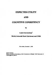
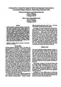
4. ILLUSTRATIVE EXAMPLES As illustrative examples, we use multi layer perceptron (MLP) neural networks and Gaussian processes (GP) with Markov Chain Monte Carlo sampling (Neal, 1996, 1999; Lampinen and Vehtari, 2001) in one toy problem (MacKay’s robot arm) and two real world problems: concrete quality estimation and forest scene classification (see Vehtari and Lampinen, 2001, for details of the models, priors and MCMC parameters). The MCMC sampling was done with the FBM1 software and Matlab-code partly derived from the FBM and Netlab2 toolbox. Importance weights for MLP networks and GPs were computed as described in Vehtari (2001, Ch. 3.2.2). 4.1. Toy Problem: MacKay’s Robot Arm The task is to learn the mapping from joint angles to position for an imaginary robot arm. Two real input variables, x1 and x2 , represent the joint angles and two real target values, y1 and y2 , represent the resulting arm position in rectangular coordinates. The relationship between inputs and targets is y1 = 2.0 cos(x1 ) + 1.3 cos(x1 + x2 ) + e1 , y2 = 2.0 sin(x1 ) + 1.3 sin(x1 + x2 ) + e2 , where e1 and e2 are independent Gaussian noise variables of standard deviation 0.05. As training data sets, we used the same data sets that were used by MacKay (1992). We used an 8-hidden-unit MLP and a GP with normal (N ) residual model. Figure 1 shows the different components that contribute to the uncertainty in the estimate of the expected utility. The variability due to having slightly different training sets in 10-fold-CV and the variability due to the Monte Carlo approximation are negligible compared to the variability due to not knowing the true noise variance. Figure 1 also demonstrates the comparison of models using paired comparison of the expected utilities. The two models are almost indistinguishable on grounds of predictive utility. 10−fold CV (90% CI) Bias in uncorrected 10−fold CV Variability due to different training sets Variability due to Monte Carlo integration
10−fold CV (90% CI) Bias in uncorrected 10−fold CV Variability due to different training sets Variability due to Monte Carlo integration MLP
MLP vs. GP
GP 0.050
0.052 0.054 0.056 Root mean square error
0.058
0.000 0.001 0.002 Difference in root mean square errors
Figure 1. The left plot shows the different components that contribute to the uncertainty, and bias correction for the expected utility (root mean square error) for MLP and GP. The right plot shows same information for the expected difference of root mean square errors.
4.2. Case Study I: Concrete quality estimation The goal of this project was to develop a model for predicting the quality properties of concrete, as a part of a large quality control program of the industrial partner of the project (J¨ arvenp¨ a¨ a, 2001). In the study, we had 27 explanatory variables and 215 samples. Here we report results for the volume percentage of air in the concrete. We tested 10-hidden-unit MLP networks and GP models with Normal (N ), Student’s tν , input dependent Normal (in.dep.-N ) and input dependent tν residual models. 1 http://www.cs.toronto.edu/~radford/fbm.software.html 2 http://www.ncrg.aston.ac.uk/netlab/
8
A. Vehtari and J. Lampinen
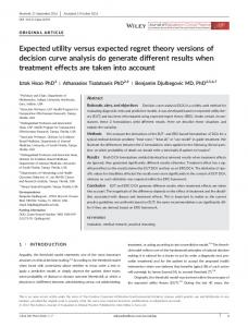
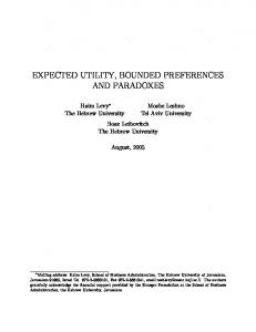
Figure 2 shows some results comparing IS-LOO-CV and k-fold-CV. IS-LOO-CV fails as importance sampling does not work well in this problem. k-fold-CV without bias correction gives overly pessimistic estimates. Figure 3 shows results comparing k-fold-CV and DIC in estimating the expected utilities and the effective number of parameters for four different noise models. DIC gives more optimistic estimates, which is probably due to using the plug-in predictive distribution and ignoring the uncertainty about the parameter values. Furthermore, since DIC provides only point estimates, it is harder to know whether the difference between models is significant
MLP − N GP − N 0.3
0.4 0.5 0.6 0.7 90%−quantile of absolute error
0.8
GP − N Effective sample size
IS−LOO−CV (90% CI) Uncorrected 10−fold−CV (90% CI) Corrected 10−fold−CV (90% CI)
Effective sample size
MLP − N 100 75 50 25 0
0
100 Data point i
200
100 75 50 25 0
0
100 Data point i
200
Figure 2. The left plot shows the comparison of IS-LOO-CV and k-fold-CV with and without bias correction. The right plot shows the effective sample sizes of the importance sampling (i) meff for each data point i (sorted in increasing order). Small effective sample sizes imply that IS-LOO-CV does not work.
With 10−fold−CV (90% CI) With DIC
With 10−fold−CV (90% CI) With DIC GP − N
GP − N
GP − in.dep. N
GP − in.dep. N
GP − tν
GP − tν
GP − in.dep. tν
GP − in.dep. tν 0.8
0.9 1 1.1 Mean predictive likelihood
60 70 80 90 100 110 Effective number of parameters p eff
Figure 3. The left plot shows the expected utility estimates with k-fold-CV and DIC. The right plot shows the effective number of parameters estimates with k-fold-CV and DIC.
4.3. Case Study II: Forest scene classification The case study here is the classification of forest scenes with MLP (Vehtari et al., 1998). The final objective of the project was to assess the accuracy of estimating the volumes of growing trees from digital images. To locate the tree trunks and to initialize the fitting of the trunk contour model, a classification of the image pixels to tree and nontree classes was necessary. Training data was 4800 samples from 48 images (100 pixels from each image) with 84 different Gabor and statistical features as input variables. We tested two 20-hidden-unit MLPs with a logistic likelihood model. The first MLP used all 84 inputs and the second MLP used a reduced set of 18 inputs selected using the reversible jump MCMC method (Vehtari, 2001). The training data has a nested structure as textures and lighting conditions are more similar in different parts of one image than in different images. If LOO-CV is used or data are divided randomly in the k-fold-CV, the training and test sets may have
Expected Utility Estimation via Cross-Validation
9
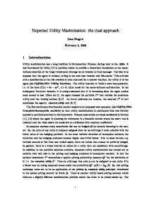
data points from the same image, which would lead to over-optimistic estimates. This is caused by the fact that instead of having 4800 independent data points, we have 48 sample images which each have 100 highly dependent data points. This increases our uncertainty about the future data. To get a more accurate estimate of the expected utility for new unseen images, the training data set has to be divided by images. Figure 4 shows the expected classification accuracy and the effective number of parameters estimated via cross-validation and (generalized) DIC. The 8-fold-CV with random data division and the DIC give overly optimistic estimates of the expected classification accuracy. The random 8-fold-CV also underestimates the uncertainty in the estimate. The DIC and the random 8-fold-CV give similar estimates of the effective number of parameters, which supports the argument that DIC assumes independent data points. If there are dependencies in the data, it is not possible to explain the difference between the model fit (the marginal posterior predictive log-likelihood) and the expected predictive log-likelihood with the effective number of parameters because this difference may be larger than the total number of parameters in the model. For example, in the case of the 18-input MLP with total of 401 parameters, this difference is about 650. With random 8−fold−CV (90% CI) With group 8−fold−CV (90% CI) With DIC
With random 8−fold−CV (90% CI) With group 8−fold−CV (90% CI) With DIC MLP − 84 inputs
MLP − 84 inputs
MLP − 18 inputs
MLP − 18 inputs 87
88 89 90 91 92 Classification accuracy %
93
200 400 600 800 1000 Effective number of parameters p eff
Figure 4. The left plot shows the expected mean predictive likelihoods computed with the 8fold-CV and the DIC. The right plot shows the estimates for the effective number of parameters computed with the random 8-fold-CV and the DIC, and the difference between the marginal posterior predictive log-likelihood and the expected predictive log-likelihood computed with group 8-fold-CV. The 84-input MLP had ptotal = 1721 and the 18-input MLP had ptotal = 401.
ACKNOWLEDGEMENTS The authors would like to thank D. Draper and D. Spiegelhalter for helpful comments on the manuscript. REFERENCES Aitkin, M. (1991). Posterior Bayes factors (with discussion). J. Roy. Statist. Soc. B 53, 111–142. Akaike, H. (1973). Information theory and an extension of the maximum likelihood principle. 2nd Int. Symp. on Inform. Theory (B. N. Petrov and F. Csaki, eds.). Budapest: Academiai Kiado. Reprinted in Breakthroughs in Statistics 1 (S. Kotz and N. L. Johnson, eds.). Berlin: Springer, 610–624. Bernardo, J. M. and Smith, A. F. M. (1994). Bayesian Theory. Burman, P. (1989). A comparative study of ordinary cross-validation, v-fold cross-validation and the repeated learning-testing methods. Biometrika 76, 503–514. Draper, D. (1996). Utility, sensitivity analysis, and cross-validation in Bayesian model-checking. Discussion of “Posterior predictive assessment of model fitness via realized discrepancies” by A Gelman et al. Statistica Sinica 6, 760–767. Draper, D. and Fouskakis, D. (2000). A case study of stochastic optimization in health policy: problem formulation and preliminary results. Journal of Global Optimization 18, 399–416.
10
A. Vehtari and J. Lampinen
Geisser, S. (1975). The predictive sample reuse method with applications. J. Amer. Statist. Assoc. 70, 320–328. Geisser, S. and Eddy, W. F. (1979). A predictive approach to model selection. J. Amer. Statist. Assoc. 74, 153–160. Gelfand, A. E. (1996). Model determination using sampling-based methods. In Markov Chain Monte Carlo in Practice (W. R. Gilks, S. Richardson and D. J. Spiegelhalter, eds.). London: Chapman and Hall, 145–162. Gelfand, A. E. and Dey, D. K. (1994). Bayesian model choice: Asymptotics and exact calculations. J. Roy. Statist. Soc. B 56, 501–514. Gelfand, A. E., Dey, D. K. and Chang, H. (1992). Model determination using predictive distributions with implementation via sampling-based methods (with discussion). Bayesian Statistics 4 (J. M. Bernardo, J. O. Berger, A. P. Dawid and A. F. M. Smith, eds.). Oxford: University Press, 147–167. Gelman, A., Meng, X.-L. and Stern, H. (1996). Posterior predictive assessment of model fitness via realized discrepancies (with discussion). Statistica Sinica 6, 733–807. Good, I. J. (1952). Rational decisions. J. Roy. Statist. Soc. B 14, 107–114. Jeffreys, H. (1961). Theory of Probability. Oxford: Oxford University Press, 3rd ed. J¨ arvenp¨ a¨ a, H. (2001). Quality Characteristics of Fine Aggregates and Controlling Their Effects on Concrete. Acta Poly. Scand. Ci 122. Helsinki: The Finnish Academies of Technology. Kass, R. E. and Raftery, A. E. (1995). Bayes factors. J. Amer. Statist. Assoc. 90, 773–795. Kong, A., Liu, J. S. and Wong, W. H. (1994). Sequential imputations and Bayesian missing data problems. J. Amer. Statist. Assoc. 89, 278–288. Lampinen, J. and Vehtari, A. (2001). Bayesian approach for neural networks – review and case studies. Neural Networks 14, 7–24. MacKay, D. J. C. (1992). A practical Bayesian framework for backpropagation networks. Neural Computation 4, 448–472. Murata, N., Yoshizawa, S. and Amari, S.-I. (1994). Network Information Criterion – Determining the number of hidden units for an Artificial Neural Network model. IEEE Trans. on Neural Networks 5, 865–872. Neal, R. M. (1996). Bayesian Learning for Neural Networks. New York: Springer Neal, R. M. (1999). Regression and classification using Gaussian process priors (with discussion). Bayesian Statistics 6 (J. M. Bernardo, J. O. Berger, A. P. Dawid and A. F. M. Smith, eds.). Oxford: University Press, 475–501. Rubin, D. B. (1981). The Bayesian bootstrap. Ann. Statist. 9, 130–134. Schwarz, G. (1978). Estimating the dimension of a model. Ann. Statist. 6, 461–464. Spiegelhalter, D., Best, N. G., Carlin, B. P. and van der Linde, A. (2002). Bayesian measures of model complexity and fit (with discussion). J. Roy. Statist. Soc. B 64, 583–639. Stone, M. (1974). Cross-validatory choice and assessment of statistical predictions (with discussion). J. Roy. Statist. Soc. B 36, 111–147. Vehtari, A. (2001). Bayesian Model Assessment and Selection Using Expected Utilities. Dissertation for the degree of Doctor of Science in Technology, Helsinki University of Technology. Vehtari, A. (2002). Discussion of “Bayesian measures of model complexity and fit” by Spiegelhalter et al. J. Roy. Statist. Soc. B 64, 620. Vehtari, A. (2003). Discussion of “Hierarchical multivariate CAR models for spatio-temporally correlated survival data” by Carlin et al. In this volume. Vehtari, A., Heikkonen, J., Lampinen, J. and Juuj¨ arvi, J. (1998). Using Bayesian neural networks to classify forest scenes. Intelligent Robots and Computer Vision XVII: Algorithms, Techniques, and Active Vision (D. P. Casasent, ed.). Bellingham: SPIE. 66–73. Vehtari, A. and Lampinen, J. (2001). On Bayesian model assessment and choice using cross-validation predictive densities. Tech. Rep. B23, Helsinki University of Technology, Finland. Vehtari, A. and Lampinen, J. (2002a). Bayesian model assessment and comparison using cross-validation predictive densities. Neural Computation 14, 2439–2468. Vehtari, A. and Lampinen, J. (2002b). Bayesian Input Variable Selection Using Posterior Probabilities and Expected Utilities. Tech. Rep. B31, Helsinki University of Technology, Finland.