Geosci. Model Dev., 8, 2067–2078, 2015 www.geosci-model-dev.net/8/2067/2015/ doi:10.5194/gmd-8-2067-2015 © Author(s) 2015. CC Attribution 3.0 License.
Experiences with distributed computing for meteorological applications: grid computing and cloud computing F. Oesterle1,* , S. Ostermann2 , R. Prodan2 , and G. J. Mayr1 1 Institute
of Atmospheric and Cryospheric Science, University of Innsbruck, Innrain 52, 6020 Innsbruck, Austria of Computer Science, University of Innsbruck, Innsbruck, Austria * née Schüller 2 Institute
Correspondence to: F. Oesterle (
[email protected]) Received: 22 December 2014 – Published in Geosci. Model Dev. Discuss.: 10 February 2015 Revised: 17 June 2015 – Accepted: 29 June 2015 – Published: 13 July 2015
Abstract. Experiences with three practical meteorological applications with different characteristics are used to highlight the core computer science aspects and applicability of distributed computing to meteorology. Through presenting cloud and grid computing this paper shows use case scenarios fitting a wide range of meteorological applications from operational to research studies. The paper concludes that distributed computing complements and extends existing high performance computing concepts and allows for simple, powerful and cost-effective access to computing capacity.
1
Introduction
Meteorology has an ever growing need for substantial amounts of computing power, be it for sophisticated numerical models of the atmosphere itself, modelling systems and workflows, coupled ocean and atmospheric models or the accompanying activities visualisation or dissemination. In addition to the increased need for computing power, more data are being produced, transferred and stored, which increases the problem. Consequently, concepts and methods to supply the compute power and data handling capacity also have to evolve. Until the beginning of this century, high performance clusters, local consortia and/or buying cycles on commercial clusters were the main methods to acquire sufficient capacity. Starting in the mid-1990s, the concept of grid computing, in which geographical and institutional boundaries only play a minor role, became a powerful tool for scientists. Foster and Kesselman (2003) published the first and most cited def-
inition of the grid: “A computational grid is a hardware and software infrastructure that provides dependable, consistent, pervasive, and inexpensive access to high-end computational capabilities”. In the following years the definition changed to viewing the grid not as a computing paradigm, but as an infrastructure that brings together different resources in order to provide computing support for various applications, emphasising the social aspect (Foster and Kesselman, 2004; Bote-Lorenzo et al., 2004). Grid initiatives can be classified as compute grids, i.e. solely concentrated on raw computing power, or data grids concentrating on storage/exchange of data. Many initiatives in the atmospheric sciences have utilised compute grids. One of the first climatological applications to use a compute grid is the Fast Ocean Atmospheric Model (FOAM) (Nefedova et al., 2006). They performed ensemble simulations of a coupled climate model on the Teragrid, a US-based grid project sponsored by the National Science Foundation. More recently, Fernández-Quiruelas et al. (2011) provided an example with the Community Atmospheric Model (CAM) for a climatological sensitivity study investigating the connection of sea surface temperature and precipitation in the El Niño area. Todorova et al. (2010) presents three Bulgarian projects investigating air pollution and climate change impacts. WRF4SG utilises grid computing with the Weather Research and Forecast Model (WRF) (Blanco et al., 2013) for various applications in weather forecasting and extreme weather case studies. TIGGE, the THORPEX Interactive Grand Global Ensemble, partly uses grid computing to generate and share atmospheric data between various partner (Bougeault et al., 2010). The Earth
Published by Copernicus Publications on behalf of the European Geosciences Union.
2068
F. Oesterle et al.: Grid computing and cloud computing
system grid ESGF (Earth System Grid Federation) is a US– European data grid project concentrating on storage and dissemination of climate simulation data (Williams et al., 2009). Cloud computing is slightly newer than grid computing. Resources are also pooled, but this time usually within one organisational unit, mostly within commercial companies. Similar to grids, applications range from services based on demand to simply cutting ongoing costs or determining expected capacity needs. The most important characteristics of clouds are condensed into one of the most recent definitions by Mell and Grance (2011): “Cloud computing is a model for enabling ubiquitous, convenient, on-demand network access to a shared pool of configurable computing resources, (e.g. networks, servers, storage, applications, and services) that can be rapidly provisioned and released with minimal management effort or service provider interaction”. Further definitions can be found in Hamdaqa and Tahvildari (2012), Vaquero and Rodero-Merino (2008) or Vaquero and RoderoMerino (2008). One of the few papers to apply cloud technology to meteorological research is Evangelinos and Hill (2008), who conducted a feasibility study for cloud computing with a coupled atmosphere–ocean model. In this paper, we discuss advantages and disadvantages of both infrastructures for atmospheric research, show the supporting software ASKALON, and present three examples of meteorological applications, which we have developed for different kinds of distributed computing: projects MeteoAG and MeteoAG2 for a compute grid, and RainCloud for cloud computing. We look at issues and benefits mainly from our perspective as users of distributed computing. Please note we describe our experiences but do not show a direct, quantitative comparison, as we did not have the resources to run experiments on both infrastructures with identical applications.
2 2.1
Aspects of distributed computing in meteorology Grid and cloud computing
Our experiences in grid computing come from the projects MeteoAG and MeteoAG2 within the national effort AustrianGrid (AGrid), including partners and supercomputer centres from all over Austria (Volkert, 2004). AGrid phase 1 started in 2005 and concentrated on research of basic grid technology and application. Phase 2, started in 2008, continued to build on research of phase 1 and additionally tried to make AGrid self-sustaining. The research aim of this project was not to develop conventional parallel applications that can be executed on individual grid machines, but rather to unleash the power of the grid for single distributed program runs. To simplify this task, all grid sites are required to run a similar Linux operating system. At the height of the project AGrid consisted of nine clusters distributed over five locations in Austria including various smaller sites with ad hoc desktop Geosci. Model Dev., 8, 2067–2078, 2015
PC networks. The progress of the project, its challenges and solutions were documented in several technical reports and other publications (Bosa and Schreiner, 2009). For cloud computing, plenty of providers offer services, e.g. Rackspace or Google Compute Engine. Our cloud computing project RainCloud uses Amazon Web Services (AWS), simply because it is the most well known and widely used. AWS offers different services for computing, different levels of data storage and data transfer, as well as tools for monitoring and planning. The services most interesting for meteorological computing purposes are Amazon Elastic Compute cloud (EC2) for computing and Amazon Simple Storage Service (S3) for data storage. For computing, so-called instances, (i.e. virtual computers) are defined according to their compute power relative to a reference CPU, available memory, storage and network performance. Figure 1 shows the basic structure of cloud computing on the right side and AGrid as a grid example on the left side. In both cases an additional layer, so-called middleware, is applied between the compute resources and the end user. The Middleware layer handles all necessary scheduling, transfer of data and set up of cloud nodes. Our middleware is ASKALON (Ostermann et al., 2008), which is described in more detail in Sect. 2.2. In the following sections, we list advantages and disadvantages of grid and cloud concepts, which affected our research most (see Table 1 for a brief overview). Criteria are extracted from literature, most notably Foster et al. (2008) containing a general comparison with all vital issues, Mell and Grance (2011), Hamdaqa and Tahvildari (2012) and Foster and Kesselman (2003). The discussed issue of security of sensitive and valuable data did not apply to our research and operational setting. However, for big and advanced operational weather forecasting this might be an issue due to its monetary value. Because the hardware and network is completely out of the end user’s control, possible security breaches are harder or even impossible to detect. If security is a concern, detailed discussions can be found in Cody et al. (2008) for grid computing, and Catteddu (2010) and Feng et al. (2011) for cloud computing. 2.1.1
Advantages and disadvantages grid
+ Handle massive amounts of data. The full atmospheric model in MeteoAG generated large amounts of data. Through grid tools like gridftp (Allcock et al., 2002) we were able to efficiently transfer and store all simulation data. + Access to high performance computing (HPC) which suits parallel applications, (e.g. Message Passing Interface, MPI). The model used in MeteoAG, as many other meteorological models, is a massive parallel application parallelised with MPI. On single systems they run efficiently; however, across different HPC clusters latencies www.geosci-model-dev.net/8/2067/2015/
F. Oesterle et al.: Grid computing and cloud computing
2069
End user Develop workflow with GUI
Askalon Middleware
Instance 1
Cluster 2
Execute Engine
Instance 2
m CPU’s
ssh job submission GRAM job submission
s CPU’s
Cluster N-1
Scheduler
Instance M-1
p CPU’s
match jobs to resources
r CPU’s
Cluster 1 Base grid Infrastructure e.g. Austrian Grid: approx. 500 CPU’s (2006) - Uni. Innsbruck - Uni. Vienna - Uni. Linz ...
Grid
Results
Submit workflow
k CPU’s
...
Cluster N q CPU’s
s CPU’s
...
Cloud provider e.g.: Amazon Lunacloud ...
Instance M
Resource Manager
r CPU’s
Cloud
e.g. via EC2 API
Figure 1. Schematic set-up of our computing environment for grid (left) and cloud (right) computing. End users interact with the ASKALON middleware via a Graphical User Interface (GUI). The number of CPUs per cluster provided by the base grid varies, whereas the instance types of cloud providers can be chosen. Execute engine, scheduler and resource manager interact to effectively use the available resources and react to changes in the provided computing infrastructure. Table 1. Overview of advantages/disadvantages of grids and clouds affecting our applications most. For a detailed discussion see Sect. 2. grids
clouds
+ Massive amounts of data + Access to parallel computing enabled high performance computing (HPC)
+ Cost + Full control of software set-up + Simple on-demand access
− Inhomogeneous hardware architectures − Complicated set-up and inflexible handling − Special compilation of source code needed
− Slow data transfer − Not suitable for MPI computing
become too high. A middleware can leverage the advantage of access to multiple machines and run applications on suitable machines and appropriately distribute parts of workflows in parallel. − Different hardware architectures. During tests in MeteoAG, we discovered problems due to different hardware architectures (Schüller et al., 2007). We tested different systems with exactly the same set-up and software and got consistently different results. In our case this affected our complex full model, but not our simple model. The exact cause is unclear, but most likely a combination of programming, the libraries and set-up down to the hardware level. − Difficult to set up and maintain as well as inflexible handling. For us, the process of getting necessary updates, patches or special libraries needed in meteorology onto all grid sites was complex and lengthy or sometimes even impossible due to operating system limitations. − Special compilation of source code. To get the most out of the available resources, the executables in MeteoAG www.geosci-model-dev.net/8/2067/2015/
needed to be compiled for each architecture, with possible side effects. Even in a tightly managed project like AGrid, we had to supply three different executables for the meteorological model, with changes only during compilation, not in the model code itself. Other typical characteristics are not as important for us. The “limited amount of resources” never influenced us as they were always vast enough to not hinder our models. The “need to bring your own hardware/connections” is also a small hindrance, since this is usually negotiable or the grid project might have different levels of partnership. 2.1.2
Advantages and disadvantages cloud computing
+ Cost. Costs can easily be determined and planned. More about costs can be found in Sect. 4. + Full control of software environment, including operating system (OS) with root access. This proved to be one of the biggest advantages for our workflows. It is easy to install software, special libraries or modify any component of the system. Cloud providers usually offer most Geosci. Model Dev., 8, 2067–2078, 2015
2070
F. Oesterle et al.: Grid computing and cloud computing
standard operating systems as images/Amazon Machine Image (AMI), but tuned images can also be saved permanently and made publicly available (with additional storage costs). + Simple on-demand self-service. For applications with varying requirements for compute resources or with repeated but short needs for compute power, simple ondemand self-service is an important characteristic. As long as funds are available the required amount of compute power can be purchased. Our workflow was never forced to wait for instances to be available. Usually our standard on-demand Linux instances were up and running within 5–10 s (Amazon’s documentation states a maximum of 10 min).
but play a less important role as resources showed to be more reliable in the cloud case. Figure 1 shows the design of the ASKALON system. Workflows can be generated in a scientist-friendly Graphical User Interface (GUI) and submitted for execution by a service. This allows for long lasting workflows without the need for the user to be online throughout the whole execution period. Three main components handle the execution of the workflow: 1. Scheduler. Activities are mapped to physical (or virtualised) resources for their execution with the end user deciding which pool of resources are used. A wide set of scheduling algorithms is available, e.g. Heterogeneous Earliest Finish Time (HEFT) (Zhao and Sakellariou, 2003) or Dynamical Critical Path - Clouds (DCPC) (Ostermann and Prodan, 2012). HEFT, for example, takes as input tasks, a set of resources, the times to execute each task on each resource and the times to communicate results between each job on each pair of resources. Each task is assigned a priority and then distributed onto the resources accordingly. For the best possible scheduling, a training phase is needed to get a function that relates the problem size to the processing time. Advanced techniques in prediction and machine learning are used to achieve this goal (Nadeem and Fahringer, 2009; Nadeem et al., 2007).
− Slow data transfer and hardly any support for MPI computing. Data transfer to and from cloud instances is slow as well as higher network latency between the instances. Only a subset of instance types are suitable for MPI computing. This limitation makes cloud computing unsuitable for large-scale complex atmospheric models. “Missing information about underlying hardware” has no impact on our workflow, as we are not trying to optimise a single model execution. “No common standard between clouds” and the possibility of “a cloud provider going out of business” is also unimportant for us. Our software relies on common protocols like ssh and adaptation to a new cloud provider could be done easily by adjusting the script requesting the instances. 2.2
2. Resource manager. cloud resources are known to “scale by credit card” and theoretically an infinite amount of resources is available. The resource manager has the task to provision the right amount of resources at the right moment to allow the execute engine to run the workflow as the scheduler decided. Cost constraints must be strictly adhered to as budgets are in practice limited. More on costs can be found in Sect. 4.
Middleware ASKALON
To make it as simple as possible for a (meteorological) end user to use distributed computing resources, we make use of a so-called middleware system. ASKALON, an existing middleware from the Distributed and Parallel Systems group in Innsbruck, provides integrated environments to support the development and execution of scientific workflows on dynamic grid and cloud environments (Ostermann et al., 2008). To account for the heterogeneity and the loosely coupled nature of resources from grid and cloud providers, ASKALON has adopted a workflow paradigm (Taylor et al., 2007) based on loosely coupled coordination of atomic activities. Distributed applications are split in reasonably small execution parts, which can be executed in parallel on distributed systems, allowing the runtime system to optimise resource usage, file transfers, load balancing, reliability, scalability and handle failed parts. To overcome problems resulting from unexpected job crashes and network interruptions, ASKALON is able to handle most of the common failures. Jobs and file transfers are resubmitted on failure and jobs might also be rescheduled to a different resource if transfers or jobs failed more than 5 times on a resource (Plankensteiner et al., 2009a). These features still exist in the cloud version Geosci. Model Dev., 8, 2067–2078, 2015
3. Execute engine. Submission of jobs and transfer of data to the compute resources is done with a suitable protocol, e.g. ssh or Globus resource allocation manager (GRAM) in a Globus environment. – System reliability. An important feature which is distributed over several components of ASKALON is the capability to handle faults in distributed systems. Resources or network connections might fail any time and mechanisms as described in Plankensteiner et al. (2009a) are integrated in the execution engine Qin et al. (2007) allowing workflows to finish even when parts of the system fail. 3
Applications in meteorology
In the following subsections, we detail the three applications we developed for usage with distributed computing. www.geosci-model-dev.net/8/2067/2015/
F. Oesterle et al.: Grid computing and cloud computing All projects investigate orographic precipitation over complex terrain. The most important distributed computing characteristics of the projects are shown in Table 3.
2071 lating an atmosphere at rest or linear orographic precipitation to test for such differences. 3.2
3.1
MeteoAG
MeteoAG started as part of the AGrid computing initiative. Using ASKALON we created a workflow to run a full numerical atmospheric model and visualisation on a grid infrastructure (Schüller, 2008; Schüller et al., 2007; Schüller and Qin, 2006). The model is the non-hydrostatic Regional Atmospheric Modeling System (RAMS; version 6), a fully MPI parallelised Fortran-based code (Cotton et al., 2003). The National Center for Atmospheric Research (NCAR) graphics library is used for visualisation. Due to all AGrid sites running a similar Linux OS, no special code adaptations to grid computing were needed. We simulated real cases as well as idealised test cases in the AGrid environment. Most often these were parameter studies testing sensitivities to certain input parameters with many slightly different runs. The investigated area in the realistic simulations covered Europe and a target area over western Austria. Several nested domains are used with a horizontal resolution of the innermost domain of 500 m and 60 vertical levels (approx. 7.5 million grid points). Figure 2 shows the workflow deployed to the AGrid. Starting with many simulations with a shorter simulation time, it was then decided which runs to extend further. Only runs where heavy precipitation occurs above a certain threshold were chosen. Postprocessing done on the compute grid includes extraction of variables and preliminary visualisation, but the main visualisation was done on a local machine. The workflow characteristics relevant for distributed computing are a few (20–50) model instances but highly CPU intensive as well as lots of interprocess communications. Results of this workflow require a substantial amount of data transfer between the different grid sites and the end user (O(200 Gb)). Upon investigation of our first runs it was necessary to provide different executables for specific architectures (32 bit, 64 bit, 64 bit Intel) to get optimum speed. We ran into a problem while executing the full model on different architectures. Using the exact same static executable with the same input parameters and set-up led to consistently different results across different clusters (Schüller et al., 2007). For real case simulations, these errors are negligible compared to errors in the model itself. But for idealised simulations, e.g. investigation of turbulence with an atmosphere initially at rest, where tiny perturbations play a major role, this might lead to serious problems. We were not able to determine the cause of these differences. It seems to be a problem of the complex code of the full model and its interaction with the underlying libraries. While we can only speculate on the exact cause, we strongly advise using a simple and quick test such as simuwww.geosci-model-dev.net/8/2067/2015/
MeteoAG2
MeteoAG2 is the continuation of MeteoAG and also part of AGrid (Plankensteiner et al., 2009b). Based on the experience from the MeteoAG experiments, we hypothesise that it would be much more effective to deploy an application consisting of serial CPU jobs. ASKALON is optimised for submission of single core parts of a workflow, which avoids internal parallelism and communication of activities and allows for the best control over the execution within ASKALON. Thus MeteoAG2 uses a simpler meteorological model, the linear model (LM) of orographic precipitation (Smith and Barstad, 2004). The model computes only very simple linear equations of orographic precipitation, is not parallelised, and has short runtime, O(10 s), even with high resolutions (500 m) over large domains. LM is written in Fortran. ASKALON is again used for workflow execution and Matlab routines for visualisation. With this workflow, rainfall over the Alps was investigated by taking input from the European Centre for Medium-Range Weather Forecasts (ECMWF) model, splitting the Alps into subdomains (see Fig. 3a) and running the model within each subdomain with variations in the input parameters. The last step combines the results from all subdomains and visualises them. Using grid computing allowed us to run many O(50 000) simulations in a relatively short amount of time O(h). This compares to about 50 typical, albeit a lot more complex runs in current operational meteorological set-ups. The workflow deployed to the grid (Fig. 3b) is simple with only two main activities: preparing all the input parameters for all subdomains and then the parallel execution of all runs. One of the drawbacks of MeteoAG2 is the very strict set-up that was necessary due to the state of ASKALON at that time, e.g. no robust if-construct yet, and the direct use of model executables without wrappers. The workflow could not easily be changed to suit different research needs, e.g. change to different input parameters for LM or to using a different model. 3.3
RainCloud
In switching to cloud computing, RainCloud uses an extended version of the same simple model of orographic precipitation as MeteoAG2. The main extension to LM is the ability to simulate different layers, while still retaining its fast execution time (Barstad and Schüller, 2011). The software stack again includes ASKALON, the Fortran-based LM, python scripts and Matplotlib for visualisation. The inclusion of if-constructs in ASKALON and a different approach to the scripting of activities, (e.g. wrapping the model executables in python scripts and calling these) allows RainCloud to be used in different set-ups. We are now able Geosci. Model Dev., 8, 2067–2078, 2015
2072
F. Oesterle et al.: Grid computing and cloud computing
Table 2. Prices and specifications for Amazon EC2 on-demand instances mentioned in this paper, running Linux OS in region EU-west as of November 2014. m1.xlarge, m1.medium and m2.4xlarge are previous generations which were used in our experiments. Storage is included in the instance, additional storage is available for purchase. One elastic compute unit (ECU) provides the equivalent CPU capacity of a ˙ 1.0–1.2GHz 2007 Opteron or 2007 Xeon processor. Instance family
Instance type
General purpose
m3.medium m3.2xlarge c3.8xlarge hs1.8xlarge t1.micro m1.xlarge m1.medium m2.4xlarge
Compute optim. Storage optim. Micro instances General purpose Memory optim.
vCPU
ECU
Memory (GiB)
Storage (GB)
Cost USD h−1
1 8 32 16 1 4 1 8
3 26 108 35 Var 8 2 26
3.75 30 60 117 0.615 15 3.75 68.4
1 × 4 SSD 2 × 80 SSD 2 × 320 SSD 24 × 2048 EBS only 4 × 420 1 × 410 2 × 840
0.077 0.616 1.912 4.900 0.014 0.520 0.130 1.840
(a)
(b)
Figure 2. Workflow of MeteoAG using the Regional Atmospheric Modelling System (RAMS) and supporting software REVU (extracts variables) and RAVER (analyses variables). Each case represents a different weather event. (a) Meteorological representation with indication which activities are parallelised using Message Passing Interface (MPI). (b) Workflow representation of the activities as used by ASKALON middleware. In addition to the different cases, selected variables are varied within each case. Same colours between the subfigures.
to run the workflow in three flavours without any changes: idealised, semi-idealised and realistic simulations as well as different settings, operational and research. Figure 4b depicts the workflow run on cloud computing. Only the first two activities, PrepareLM and LinearModel have to be run, the others are optional. This workflow fits a lot of meteorological applications as it has the following building blocks: – preparation of the simulations (PrepareLM); – execution of a meteorological model (LinearModel); – post-processing of each individual run, e.g. for producing derived variables (PostProcessSingle); Geosci. Model Dev., 8, 2067–2078, 2015
– post-processing of all runs (PostprocessFinal). All activities are wrapped in Python scripts. As long as the input and output between these activities are named the same, everything within the activity can be changed. We use archives for transfer between the activities, again allowing different files to be packed into these archives. The operational set-up produces spatially detailed, daily probabilistic precipitation forecasts for the Avalanche Service Tyrol (Lawinenwarndienst Tirol) to help forecast avalanche danger. Figure 4a shows the schematic of our operational workflow. Starting with data from the ECMWF, we forecast and visualise precipitation probabilities over Tyrol with a spatial resolution of 500 m. Additionally, research type www.geosci-model-dev.net/8/2067/2015/
F. Oesterle et al.: Grid computing and cloud computing
2073
LinMod:Make_NameList
LinMod:Prod_NcFiles parallel
(a)
(b)
Figure 3. Set-up and workflow of MeteoAG2 using the linear model (LM) of orographic precipitation. (a) Grid set-up of experiments in MeteoAG2 with dots representing grid points of the European Center of Medium Range Weather Forecast (ECMWF) used to drive the LM. Topography height in kilometres a.m.s.l. (b) Workflow representation of the activities as used by ASKALON. Activity MakeNML prepares all input sequentially. ProdNCfile is the main activity with the linear model run in parallel on the grid. Panel (a) courtesy of Plankensteiner et al. (2009b).
Data from global forecast model ECMWF
daily during winter, whereas research types are run in bursts. Data usage within the cloud can be substantial O(500 Gb) with all flavours, but with big differences of data transfer from the cloud back to the local machine. Operational results are small, of the order of O(100 Mb), while research results can amount to O(100 Gb), influencing the overall runtime and costs due to the additional data transfer time.
PrepareLM
Extract at predefined grid points Split Alps in subdomains
LinearModel
Modify each subdomain • higher resolution (500m)
PostProcessSingle
• vary input variables parallel
Calculate precipitation for each domain/input variable Extract Calculate probabilities Visualize
4 4.1
Costs, performance and usage scenarios Costs
PostProcessFinal
Send to LWD
(a)
Cloud
(b)
Figure 4. Workflow of RainClouds operational setting for the Avalanche Warning Service Tyrol (LWD) using the double layer linear model (LM) of orographic precipitation. Input data from the European Center for Medium Range Weather Forecast (ECMWF). (a) Meteorological flow chart with parts not executed on cloud (in red). (b) Workflow with activities as used by ASKALON. Same colours between subfigures.
experiments are used to test, explore and run experiments with new developments in LM through parameter studies. Our workflow set-ups vary substantially in required computation power as well as data size. The operational job is run www.geosci-model-dev.net/8/2067/2015/
To define the exact costs for a dedicated server system or the participation in a grid initiative is not trivial, and often even unknown to the provider; we contacted several of them, but due to complicated budgeting methodologies the final costs are not obvious. Greenberg and Hamilton (2008) discussed costs for operating a server environment for data services from a provider perspective, including servers, infrastructure, power requirements and networking. However, the authors did not include the cost of human resources for, e.g., system administration. Patel and Shah (2005) included human resources and establish a cost model for set-up and maintenance of a data centre. Grids may have different and negotiable levels of access and participation, with varying associated costs to the user. Some initiatives, e.g. PRACE (Guest et al., 2012), offer free access to grid resources after a proposal/review process.
Geosci. Model Dev., 8, 2067–2078, 2015
2074
F. Oesterle et al.: Grid computing and cloud computing
Table 3. Overview of our projects and their workflow characteristics. Project
MeteoAG
MeteoAG2
RainCloud
Type
grid
grid
cloud
Meteorological model
RAMS (Regional Atmospheric Modeling System)
single layer linear model of orographic precipitation
double layer linear model of orographic precipitation
Model type
complex full numerical model parallelised with Message Passing Interface (MPI)
simplified model
double model
Parallel runs
20–50
approx. 50 000
> 5000 operational, > 10 000 research
Runtime
several days
several hours
1–2 h operational/