Eurographics/ ACM SIGGRAPH Symposium on Computer Animation (2009) E. Grinspun and J. Hodgins (Editors)
Experiment-based Modeling, Simulation and Validation of Interactions between Virtual Walkers Julien Pettré1 Jan Ondˇrej1 Anne-Hélène Olivier 2 Armel Cretual 2 Stéphane Donikian1 1 Bunraku 2 M2S,
team, IRISA / INRIA-Rennes, France UEB, Université de Rennes 2, France
Abstract An interaction occurs between two humans when they walk with converging trajectories. They need to adapt their motion in order to avoid and cross one another at respectful distance. This paper presents a model for solving interactions between virtual humans. The proposed model is elaborated from experimental interactions data. We first focus our study on the pair-interaction case. In a second stage, we extend our approach to the multiple interactions case. Our experimental data allow us to state the conditions for interactions to occur between walkers, as well as each one’s role during interaction and the strategies walkers set to adapt their motion. The low number of parameters of the proposed model enables its automatic calibration from available experimental data. We validate our approach by comparing simulated trajectories with real ones. We also provide comparison with previous solutions. We finally discuss the ability of our model to be extended to complex situations. Categories and Subject Descriptors (according to ACM CCS): I.3.7 [Computer Graphics]: Animation; I.6.4 [Simulation and Modeling]: Model Validation and Analysis; I.6.5 [Simulation and Modeling]: Model Development; Keywords: steering method, collision avoidance, interaction
1. Introduction The computer animation community put in a great deal of effort to provide virtual humans with autonomy of locomotion. Despite the apparent simplicity of this everyday task, simulating locomotion in a realistic manner is complex, especially when virtual walkers are moving in environments made of many static and dynamic obstacles. A large body of prior work suggests that simulating interactions between virtual walkers in a realistic manner is particularly difficult.
ers’ motion, which is naturally error-prone. These first two kinds of factors, related to physics and perception, are obviously important during human interactions, but secondary factors also need attention. First, sociological and cultural factors influence human reaction according to some tacit rules (deviating preferably to the left or to the right, avoiding elderly people more carefully, etc.). Psychological factors are also involved: people walk according to their mental state (hurrying, wandering). They are capable of moving in an expressive manner to objectify this internal state.
An interaction occurs between walkers when a reciprocal influence is observed on their respective trajectory: each one adapts its own motion in order to avoid the others. Understanding and simulating interactions between humans is complex due to the possibly high number of factors involved. Human locomotion is generally driven by a goal to reach, while it is constrained by physical and biomechanical factors. In addition, environmental factors - such as the presence of obstacles - set supplementary constraints. Trajectory adaptations are based on the perception humans have of oth-
Our motivation is to achieve realistic simulation of interactions between walkers. Our objective is first to better understand how real humans behave in such situations. Our results allow us to discuss several assumptions which were formulated to build existing computational models (developed by both the crowd simulation and computer animation communities). We elaborate a new model that better fits our experimental observations. Our approach is however based on two major assumptions. First, a complex interaction that involves several walkers simultaneously can be described as a
Copyright © 2009 by the Association for Computing Machinery, Inc. Permission to make digital or hard copies of part or all of this work for personal or classroom use is granted without fee provided that copies are not made or distributed for commercial advantage and that copies bear this notice and the full citation on the first page. Copyrights for components of this work owned by others than ACM must be honored. Abstracting with credit is permitted. To copy otherwise, to republish, to post on servers, or to redistribute to lists, requires prior specific permission and/or a fee. Request permissions from Permissions Dept, ACM Inc., fax +1 (212) 869-0481 or e-mail
[email protected].
SCA 2009, New Orleans, LA, August 1–2, 2009. © 2009 ACM 978-1-60558-610-6/09/0008 $10.00
190
Pettré et al. / Experiment-based Modeling, Simulation and Validation of Interactions between Virtual Walkers
combination of pair-interactions involving two walkers only. Second, physical and perceptual factors are preponderant. Secondary factors are then to be taken into account in future works. As a result, we first focus our study on interactions to the two-walker case only. We however describe how the proposed model can handle multiple interactions. Understanding how humans combine pair-interactions to solve complex ones is discussed in this paper, but certainly deserves a complete study. Our contribution is threefold. Our primary contribution is a model for solving interactions between virtual walkers, presented in Section 4. The model is elaborated from experimental observations of real interactions between walkers, which sets our second contribution. Our experimental data are made available to the research community. Our third and final contribution is to propose a quantitative evaluation of our model results. This evaluation enables an objective assessment of simulated trajectories, as compared with real data, or ones resulting from previous solutions. The remainder of this paper is organized as follows: in Section 2, we review prior work in modeling interactions. Section 3 describes our experimental results. The model we elaborated from experiments is described in Section 4. Comparison of our model results with previous techniques is detailed in Section 5. Finally, we discuss limitations and possible extensions of our model to answer complex situations in Section 6, before concluding. 2. Related Work Mainly three research fields addressed the problem of interactions between walkers. First, cognitive sciences studied the influence of obstacles (static or moving) on human locomotion. Their experiments demonstrated that humans combine notions of time, distance and velocity to avoid collisions. The second field focused on crowd simulation. Crowd simulators mainly aim at studying the impact of numerous human-human and obstacle-human interactions on the global circulation of many walkers. Their main objective is to achieve realistic simulations at a macroscopic level, even though solutions are often based on microscopic models. The third field is Computer Animation which needs for believable individual locomotion trajectories and developed specific approaches to simulate interactions. Two main classes of solutions exist. First ones are based on steering methods: they are general and efficient, however, evaluating their level of realism is still an open question. The latter class of solutions relies on a database of captured real interactions, reused in simulations to imitate how real humans solve interactions. A high level of realism is intrinsically obtained; nevertheless, these solutions’ validity domain is limited to the database content. Time-to-collision and personal space. Avoiding collisions is a spatiotemporal problem. Cognitives sciences divided its
temporal and spatial dimensions into two different notions: the time-to-contact TTC, and the personal space. According to Cutting and colleagues [CVB95], humans avoid collisions by answering two successive questions: will a collision occur? When will this collision occur? Answers result from the visual perception of their environment and of the moving or stationary obstacles. Lee [Lee76] and Trésilian [Tré91] demonstrated that the optical flow generated from the visual perception of a moving object is sufficient to directly evaluate TTC. The real nature of information used by humans to evaluate TTC is still an open question; however, humans adapt their motion to avoid collisions in order to preserve admissible TTC. Velocity, distance and time are intrinsically linked together. As a result, TTC can also be interpreted as a preserved distance between humans and obstacles, giving rise to the personal space notion. Personal space can be defined as a safety area preserved by walkers around them. The personal space gives walkers enough time to react to an unexpected moving obstacle appearing in their perception field. Gérin-Lajoie and colleagues [GLRM05] experimentally measured the personal space’s shape and dimensions. They found the personal space is elliptic, as intuitively imagined by Goffman [Gof71]. The novelty of this study is to focus on personal space measurement while moving. However, the experimental process was based on the interaction between a human walker and a moving manikin mounted on an overhanging rail. Reactive approaches. Solving interactions is certainly a crucial component of crowd simulation. Helbing’s social forces model is probably the most popular approach [HM95]. The model was later revisited and calibrated for specific situations [HBJW05], or integrated into a software platform in order to solve well-known artifacts [PAB07]. In this model, virtual walkers are modeled as velocity-controlled particles undergoing a sum of acceleration forces with an analogy to Physics. Interactions are modeled as repulsive forces between walkers, and expressed as a function of their relative distance. Treuille and colleagues [TCP06] also make an analogy to Physics, but formulate interactions as a minimization problem. Walkers’ motion is deduced from a potential field, whose dynamic component results from a repulsion emitted by walkers. Walkers avoid each other implicitly, interactions are not explicitly modeled. In [HLTC03], interactions between humans are modeled as a mass-spring-damper system: stiffness and viscosity terms change with respect to relative distance between walkers. Anticipated collision avoidance. The steering behaviors introduced in [Rey99] enable interaction solving with anticipation. The unaligned collision avoidance behavior extrapolates walkers’ trajectories - assuming that their velocity is constant - and checks for collisions in a near future. A reactive acceleration is computed for both walkers, in the direction opposite from the one of the future colli-
Pettré et al. / Experiment-based Modeling, Simulation and Validation of Interactions between Virtual Walkers
sion. Van den Berg and colleagues extend the Reciprocal Velocity Obstacle principle from Robotics [vdBPS∗ 08]. Similarly to Reynolds’ steering, this technique enables collaborative interaction solving with anticipation. Finally, Paris and colleagues [PPD07], inspired by Feurtey [Feu00], solves the problem from an egocentric perspective (i.e., walkercentered). In this approach, perceived neighbors’ motion is also linearly predicted; an admissible velocity domain for each walker is deduced. A cost function is used to compute a specific velocity command belonging to the admissible ones. More recently, Kapadia and colleagues proposed an egocentric anticipative model in [KSHF09]. Imitating humans. Several solutions appeared in the literature taking advantage of motion capture or video tracking technologies to create databases of real interactions [MH04]. In [LCHL07], relative motions and positions between virtual humans are related to behaviors: this approach applies to the collision avoidance problem, but more generally enables behavioral crowd animation. In [LCL07], the authors solve interactions occurring in a simulation by retrieving the most similar example from the database; however, controllability and efficiency problems rise. Both of these problems are solved in [TLP07]: walkers are described using a statevector, whilst a captured motion is modeled as a state-vector change. Given a user-defined state command, a motion sequence is found to reach the desired state in a near-optimal manner. Some components of the state-vector are used to describe interactions with one neighbor walker: this technique is thus able to solve interactions. Our approach. The experimental study proposed in the next section allows us to describe how humans solve collisions. We demonstrate that the adaptations are not purely reactive and cannot only be modeled as a function of the distance between them. It is however possible that this assumption becomes true in the case of crowded areas where walkers have numerous and intensive interactions. Nevertheless, a realistic simulation and animation of virtual walkers in the general case need anticipation. We have mentioned existing solutions to anticipate a reaction. However, several questions remain: some approaches anticipate a reaction at constant distance or time to collision, others immediately when interaction is detected. Our experiments demonstrate that interactions start with an observation period of time, which allows humans to estimate other’s motion accurately enough before reacting. Our model accounts for perceptionerrors in order to evaluate when reactions occur. Moreover, previous solutions assume velocity is constant before interaction, which enables linear extrapolations of trajectories. We discuss and address the more complex case where walkers are accelerating when interactions are initiated. Concerning imitation techniques, their main advantage is their intrinsic realism. However, two main drawbacks limit their application. First, efficiency does not always enable realtime simulation. Second, their validity domain is restricted
191
Figure 1: Illustration of the proposed experimental protocol.
by the content of example databases. Furthermore, some of these techniques do not apply to multiple interactions. About steering methods, the obtained level of realism has not always been evaluated. Brogan and Johnson proposed evaluation metrics to assess simulated trajectories [BJ03]. Singh and colleagues [SNK∗ 08] proposed a framework to evaluate the ability of steering methods to address interactions among obstacles. We propose an objective evaluation of our results based on real data.
3. Experimental Study Objectives Our objective is here to describe how humans solve pair-interactions. We choose to observe interactions under protocol-controlled conditions, in order to diminish and more important, to maintain constant between each experimental sample - the role of secondary factors: we focus our attention on physical and perceptual factors only. Accurate measures of motion adaptations are desired, and we choose to use a motion capture system to acquire experimental data. Protocol The proposed experimental protocol is illustrated in Figure 1. At the start of each experiment, 4 participants stay still at each corner of a square experimental area. We randomly give 2 of the 4 participants the simultaneous order to walk toward the opposite corner (along each diagonal), the 2 others leave the experimental area. Start signals are given to participants by network-synchronized computers. Participants have orthogonally intersecting paths and synchronized trajectories: they are likely to interact, but not necessarily. Initial conditions of interactions change for each experiment because participants are asked to walk at their own comfort speed. Occluding walls prevent participants to observe each other before reaching their comfort speed. Our experimental square is 15m long, interaction area is 10m long. We randomize the selection of participants, so that they cannot anticipate the direction from which one may appear. 30 subjects have taken part in this experiment. We recorded 429 experimental samples.
192
Pettré et al. / Experiment-based Modeling, Simulation and Validation of Interactions between Virtual Walkers
Figure 2: left: average adaptation over all experiments made by participant passing first, function of minimum predicted distance and normalized time to interaction. right: average adaptation over all experiments made by participant giving way, function of minimum predicted distance and normalized time to interaction.
Figure 3: left: minimum predicted distance for one experiment, function of normalized time to interaction. Three successive periods of time are observed: observation, reaction, and regulation. right: density of minimum predicted distance trajectories over all experiments, function of normalized time to interaction
Method The trajectory was established from the mean of the two shoulder markers: P(x, y). Velocity is noted V = dP/dt and acceleration is noted A = dV /dt. We note θ the velocity vector direction, and v its norm. We check that lateral velocities can be neglected, and assume locomotion is non-holonomic in our case [ALHB08]. Data are filtered to remove noise and reduce the effect of natural oscillations (Butterworth low-pass second order filter, 1Hz cutoff frequency, zero phase shift). Trajectories are decomposed into three periods of time: participants start walking during the initial phase, during which they reach their comfort speed. The interaction phase starts when participants are able to see each other (with respect to occluding walls), at time t = tvis . The time when the distance between participants is minimal is called the interaction time tint . Finally, for t > tint , participants head again for their goal during the recovery phase. Our study is focused on the interaction phase, for tvis < t < tint . In the absence of interaction, participants have constant velocity inside the interaction area. Their trajectory can be predicted linearly as follows:
ttin ranges from 1 to 0, respectively corresponding to the normalized time at which the interaction phase starts, and next, ends.
τ pred (t, u) = P + (u − t)V,
(1)
τ pred is the predicted trajectory from instantaneous position and velocity at time t. Parameter u > t corresponds to the future time. For any time t belonging the interaction phase, we are able to predict the distance at which they would meet if no adaptation is made (the minimum predicted distance mpd): −−−−−−−−−−−−−−−→ mpd(t) = min kτ pred,1 (t, u)τ pred,2 (t, u)k, (2) u>t
where τ pred,1 and τ pred,2 are the predicted trajectories for each of the participants at time t. As participants walk at their own comfort speed, initial interaction conditions change for each experiment. This results in a variety of initial mpd(t = tvis ) values over all our experiments. Finally, in order to enable direct inter-experiments comparison, we normalize the duration of the interaction phase and define the normalized time-to-interaction ttin as follows (average duration of interaction phase over all experiments is 4 s.): ttin (t) = (tint − t)/(tint − tvis ),
(3)
Minimum predicted distance as a motion adaptation criterion. As participants’ motion is linear in absence of interaction, we simply detect motion adaptation by direct measuring of accelerations. We define thus the adaptation quantity a(t) as follows: q a(t) = kA(t)k = kV˙ (t)k = v˙2 (t) + θ˙ 2 (t).v2 (t). (4) Previous studies state that walkers first determine whether a collision will occur, and react (or not) accordingly. As a result, adaptations are to be detected for low mpd values only. Figure 2 plots participants’ adaptation averaged over all our experiments, in function of mpd (on vertical axis) and ttin (horizontal axis). Adaptations of the participant passing first and of the one giving way are plotted separately (respectively the top and bottom plot). A strong relation between adaptation and mpd is effectively observed: when mpd > 1m, almost no acceleration is detected. Note that adaptations at low normalized time values (ttin < 0.1) correspond to the initiation of the recovery phase. Three successive stages. The left plot of Figure 3 shows the evolution of mpd in time for one single experiment. At the beginning of interaction phase, we observe 0.1m < mpd < 0.35m: collision is predicted (mpd is effectively a body center-to-center distance). mpd remains low for half of the interaction phase. We call this first stage the observation period. Following this, mpd is increased during the reaction period to an acceptable value of 1m, enabling collision avoidance: participants necessarily adapt their motion to increase mpd. However, we cannot determine from this plot only if adaptation is made by one participant or both. Finally, mpd is maintained during the regulation phase. mpd gives a clear temporal description of interactions. In order to obtain a statistical overview of interaction solving, we cumulate mpd trajectories for all experiments, and plot the density of trajectories: the result is given at the right of Fig-
Pettré et al. / Experiment-based Modeling, Simulation and Validation of Interactions between Virtual Walkers
193
ure 3. Note that we later use the density plot to qualitatively compare simulated and real data. We conclude that the observation period statistically takes place for 1 > ttin > 0.8, which means during the first 0.8s of the interaction phase. Reaction period averagely lasts for 1.6s (ttin ∈ [0.8, 0.4]). Finally, during the remaining time (1.6s until ttin = 0, i.e., t = tint ) motion is regulated to maintain admissible mpd values. Note that mpd becomes closer to the distance between participants when the interaction phase is ending. As a result, we can see that the average distance at which participants meet is distributed around 0.8m. The existence of the regulation period of time confirms interactions are solved with anticipation. A role-dependent adaptation. Figure 2 separately plots the adaptations made by each of the two participants. We observe that both make adaptations, however, the first participant passing is clearly making less efforts. In conclusion, interaction is solved collaboratively, but asymmetrically. Further analysis also reveals different strategies: the first participant mainly adapts his velocity, whereas the one giving way combines velocity and orientation adaptations. This asymmetry confirms the notion of the personal space: in order to preserve this space, the participant giving way needs to make larger avoidances. Adaptation is error-prone. A common experience we all have had while walking is to get close to colliding with someone after successive hesitations on how to avoid him. We could observe such hesitations: mpd(t) value is lowered in time instead of being increased. Antinomic adaptations occur only when mpd is initially close to 0m. In such a case, the role of each participant is not clearly predictable. The observation period then becomes longer, and reaction is delayed. Do participants refine their motion estimation to determine their role? Nevertheless, such cases provoke the acceleration peak that can be seen in Figure 2, right plot, for ttin ≈ 0.4 and mpd ≈ 0m. The density plot however reveals that such cases remain rare.
4. A model for solving interactions between walkers We elaborated a model for solving interactions between virtual walkers from our experimental observations. Our model is based on an egocentric representation of walkers’ relative motion. In the following part, we describe how our model solves pair-interaction. Next, we describe a calibration technique to compute realistic model parameters from real interaction data. Finally, the case of multiple interactions is addressed in Section 4.3.
4.1. A Model for Solving Pair-Interactions Overview. An interaction is solved for each of the two involved virtual walkers independently. Walkers are modeled
Figure 4: left: Illustration of the components of the proposed model. Solution is based on an egocentric representation of the interaction situation. right: Step 2 and 3 of a Model Iteration: walker’s role is deduced from the position of I relatively to the decision line. A solution velocity is computed in order for I to exit the interaction area.
as velocity-controlled moving points. Our description is supported by the example introduced in Figure 4, left. Two walkers walk straight forward at comfort velocity toward their goal, their trajectories are secant. We note R the reference walker for which the model is controlling the motion, displayed at the bottom of the figure. The perceived walker on the top-right of the figure is noted P. Our approach is based on several components described below. Model components The first step of our solution consists in computing the egocentric representation of the interaction situation, as illustrated in Figure 4. We first compute P’s position and velocity relatively to R. We consider thus the local coordinate system centered and oriented on the reference walker R. P’s relative position is noted PP/R , and relative velocity is computed as follows: VP/R = VP/W +VW/R ,
(5)
where VP/W is the velocity of P relatively to the world W, and VW/R the relative motion of W relatively to R (simply deduced from absolute velocity vector: VW/R = −VR/W ). The reference walker’s desired velocity Vd is directly deduced from its goal. Vd is oriented toward this goal, its norm is the reference walker’s comfort velocity vc . The constant vc is thus an individual parameter. Vd is then expressed in the local coordinate system as a desired world velocity relatively to the reference walker: VdW/R = −Vd . In the case presented in Figure 4, the reference walker is walking at the desired velocity as no adaptation has been made yet. As a result, desired velocity and current velocity coincide. A personal area is set around the reference walker. Personal area has a kite shape. The kite approximates the elliptic shape experimentally measured by [GLRM05], but is
194
Pettré et al. / Experiment-based Modeling, Simulation and Validation of Interactions between Virtual Walkers
mathematically much simpler to handle. The kite allows the reference walker to keep more space available in front of it than in its back and on its sides. Note that the personal area here maintains a center-to-center distance between walkers. The kite’s dimension on each side and on the back is 0.8m and velocity-dependent in front of it (where ut is the unit of time): l = 0.8 + 0.4v.ut .
(6)
T1 and T2 are the tangents to the personal area passing by PP/R . These tangents delimit an area called interaction area (colored in light green in Figure 4). We also define the interaction point I as follows: I = PP/R + ut VP/W + ut VdW/R .
(7)
Our technique is mainly based on the position of I relatively to the interaction area: virtual walkers play on this position to solve an interaction. I results from the relative motion of P to R, however, each virtual walker can only act on the self-motion component of this relative velocity. Our experiments demonstrate the importance of motion perception to explain the interaction temporal structure. As a result, we model the interaction point location relatively to R as prone to errors. We only take into account velocity and orientation perception errors (respectively noted εv and εθ ), as they result from position integration in time since interaction initiation. We neglect position and self-motion perception errors. We model perception errors by transforming the I point into a locus: Ilocus . Errors are dependent on the observation time since the reference walker is perceiving P: the longer the observation time, the lower the errors. We compute εv and εθ , as functions of time-to-interaction tti, as follows: tti = arg min kPP/R + k.VP/R k, k
tint )γv ), tint + tti t εθ = βθ .(1 − ( int )γθ ), tint + tti εv = βv .(1 − (
(8) (9)
R’s personal area. We are then in the situation illustrated by Figure 4, right image. (a detailed-view of Figure 4 where R is not represented anymore). The goal of the following steps is to move I on the limits of the interaction area. In the opposite case, the model iteration stops here. Step 2 - What is the reference walker’s role? By the interaction point definition (cf. Equation 7), the reference walker can modify I’s position by adapting its desired velocity, which becomes the solution velocity. In order to solve the interaction in an optimal manner, I has to be on the limit of the interaction area: I ∈ T1 or I ∈ T2 . These two solution domains respectively correspond to two different roles: passing first or giving way. Decision is taken from the relative position of I to the decision line. In the case of Figure 4, right, I is on the side of T1 . Step 3 - Computing a solution velocity. We want I ∈ T1 (T2 when giving way), the solution velocity VsolW/R has to verify the following condition: PP/R + ut VP/W + ut VsolW/R ∈ T1 .
(11)
Infinity of solutions exists. We represent 3 of them in Figure 4, right, parameterized by α. Vsol (α = 0) corresponds to a pure orientation adaptation. Vsol (α = 1) corresponds to a pure velocity adaptation. Finally, Vsol (α = 0.5) corresponds to a combination of velocity and orientation adaptation (by orthogonal projection of I on T1 ). We thus introduce a new parameter α which defines the avoidance strategy of the reference walker. We set the default value: α = 0.5, this parameter is later calibrated from real data. Note that the personal area induces asymmetry in the model. When choosing the T2 solution domain, (i.e., when giving way) more adaptation is required, and I reaches the limits of the interaction area later. It is even possible that no adaptation is required for the first walker passing, whilst the one giving way detects a need for adapting its motion. This property is correlated to our experimental observations.
(10)
where tint is the time elapsed since P is perceived. βv , γv , βθ and γθ are parameters to be calibrated from real data as explained in the last paragraphs of this section. Default values are: βv = 0.5, βθ = 0.5, γv = 0.25, γθ = 0.25. We model Ilocus as a rectangle aligned on the P’s velocity vector VP/W . Its length (in the direction of VP/W ) is εv and its width (orthogonally to VP/W ) is εθ (see Figure 4). Finally, we define the decision line which joins R and P. We now describe the successive steps of one model iteration. Model Iteration Our model works according to the three following steps. Step 1 - Is adaptation required? If Ilocus is fully contained in the interaction area, then R has an accurate enough estimation of P’s motion to be sure they will pass at a too low distance. Indeed, the extrapolated P’s trajectory is crossing
4.2. Model Calibration A walker’s behavior is controlled by the five model parameters. α determines the walker’s avoidance strategy while βv , γv , βθ and γθ control perception error evolution in time. We provide default values for each parameter above. We now propose to use the Maximum Likelihood Estimation (M.L.E.) technique [HS98] to calibrate our model from experimental samples. Briefly, this method consists of successive testing of different parameter sets. The one leading to the best match between real and simulated trajectories is identified. We initialize simulations from the measured experimental conditions (i.e., relative position and comfort velocities at the initiation of the interaction phase). More precisely, we search for the parameter set p(α, βv , γv , βθ , γθ ) so that the likelihood estimator L(p) is maximum: n
pˆ = arg max L(p), where: L(p) = ∏ f p (δi ), p
i=0
(12)
Pettré et al. / Experiment-based Modeling, Simulation and Validation of Interactions between Virtual Walkers
(a) Uncalibrated model
(b) Calibrated model
(c) RVO model
(d) Reynolds’ model
195
(e) Helbing’s model
Figure 5: A direct comparison between real interaction (red trajectories) and simulated interaction (blue trajectories) for models.
with δi the error between the experimental position Pe at time i and the simulated position Ps for an identical time (Manhattan distance is used): −−→ δi = kPePsk1 ,
(13)
f p (δ) is the probability function of a normal distribution N (µ, σ2 ): 2 1 − (δ−µ) f p (δ) = √ e 2σ2 . 2πσ
(14)
Figure 5 illustrates the model calibration results. All plots show real trajectories (in red) superimposed with simulated ones (in blue). Simulated and real positions at identical times are linked by black line segments. The plot (a) is obtained from the uncalibrated version of our model, using the default parameter values. The plot (b) is obtained after calibration. In the latter case, perception errors are better estimated, allowing the model not to anticipate reaction too early. As a result, reaction is delayed and needs to be stronger: simulated adaptation more accurately corresponds to real data. In order to enable comparison to previous solutions, we also provide simulated data using van den Berg’s model [vdBPS∗ 08] (using the RVO library implementation), Reynold’s steering behavior [Rey99] (using the OpenSteer implementation) and Helbing’s model [HM95]. Plot (c) (RVO model) reveals the need of the asymmetrical personal area. Because of the circular representation, the correction of the walker passing second to its velocity is small. We also compare our results to the Reynolds’ technique because the assumptions used in this solution meet several of our experimental observations: reactions are anticipated and collaborative. However, walkers have symmetric reactions, and anticipation time is near-constant (just lightly randomized). However, this value is relatively correct in the case of our initial conditions. We finally choose the Helbing’s model because of the large interest showed in his approach, and the many existing variants. We further evaluate and validate our model in the following section, in comparison to these three approaches.
Figure 6: left: Step 3 is modified to solve multiple interactions. The velocity domains U1 and U2 contain all possible solution velocities for 0 ≤ α ≤ 1. right: Step 4 and 5: the reference walker R needs to avoid a collision with perceived walkers P1 and P2 . At the end of step 3, S contains 4 velocity domains: S = {U11 ,U12 ,U21 ,U22 } (orange color). After step 0 0 0 4, S’ = { U11 , U21 , U22 } (blue color), whilst U12 is dropped. The solution velocity, closest to the current one, Vsol belongs to U21 but due to the presence of P3 , this solution is rejected and the final solution velocity Vsol belongs to U22 .
4.3. Multiple Interactions In the previous section, we describe and calibrate our interaction model from the pair-interaction case perspective. We are then able to handle sparsely populated environments where a walker is usually avoiding one or few other walkers at long distance without need for further computation. In this section, we describe how our model is able to solve simultaneous multiple interactions in more densely populated environments. Two supplementary steps - step 4 and step 5 are required to address such situations. Similarly to the pair-interaction case, steps 1 to 3 are processed for each of the n perceived walker Pi , i = 1, .., n. Note that, for each pair-interaction, steps 2 and 3 run only
196
Pettré et al. / Experiment-based Modeling, Simulation and Validation of Interactions between Virtual Walkers
fig. 5 L(p) mean L(p)
calibr. model
uncal. model
RVO model
Reynolds’ steer.
Helbing’s model
0.285
0.056
0,001
0.004
1.3 10−15
0.214
0.165
0.14
0.047
0.004
Table 1: values of the likelihood function using different simulation models. First results correspond to the example given Figure 5. Second results are mean values over 429 simulations corresponding to each of the available experimental sample.
if the corresponding Ilocus is inside the interaction area. Step 3 is however slightly modified. Instead of computing Vsol according to one specific α value, we compute two velocity domains Ui1 ∈ Ti1 , Ui2 ∈ Ti2 respectively for 0 ≤ α ≤ 1. Ui1 and Ui2 are shown in Figure 6, left. Result is a set of solution velocity domains: S = {Ui1 ,Ui2 } with i = 1, .., m. Note that m < n because some of the perceived walkers have no interaction with the considered reference walker. Real humans have a limited capability of considering several interactions simultaneously, we arbitrarily limit m ≤ 7. step 4 - Merging solution velocity domains. For each interacting perceived walker, i.e., for i = 0 to m, we compute the parts of the corresponding solution velocity domain Ui1 and Ui2 not intersecting the interaction areas corresponding to any other considered walker. We thus compute a merged solution velocity domain S0 which contains reduced velocity domains Ui10 and Ui20 , computed as follows: Ui10 = Ui1 −Ui1 ∪ I j , and Ui20 = Ui2 −Ui2 ∪ I j ,
(15) th
where I j is the interaction area corresponding to the j perceived walker, j = 0..m, and j 6= i. step 5 - Rating velocity domains. In case S0 is empty, we set Vsol = 0. In the opposite case, each velocity belonging S0 successfully solves all the considered interactions. However, they may lead to new interactions with nearby walkers, yet unconsidered. To diminish the number of interactions induced by the retained solution velocity, each possible solution is envisaged. We retain the solution velocity Vsol that minimizes the number of new interactions with walkers (i.e., not considered in the S interaction set). Steps 4 and 5 are illustrated in Figure 6, right. Note that P3 is not interacting with R at this precise simulation step, but makes R preferably avoiding P1 and P2 by turning to the right in order for him to not start interacting with P3 . 5. Results Quantitative model evaluation. The likelihood function L(p) can be directly used as a metric for a quantitative evaluation of our model results. Moreover, this function can also be evaluated for any simulated data which enables compar-
ison between different approaches. Table 1 provides the obtained likelihood function value using: first, our calibrated model, second, our model using default parameter values, third, RVO model, fourth, Reynolds’ steering behavior and finally, Helbing’s model. The first line of results in Table 1 is computed from the example presented in Figure 5. The second line provides the mean value of the likelihood function computed over all the 429 available experimental samples. The higher the likelihood value, the more realistic the results. The obtained likelihood for the calibrated model is obviously higher than the one with default parameters value. Likelihood of the uncalibrated model is only slightly better than RVO model. However, this approach is not able to correctly simulate a large variety of cases, especially due to the near-constancy of anticipation times. Furthermore, adaptations are symmetrically made by the two walkers. Reynolds’ model is worse than previous two and has the same disadvantages as the RVO model. In the case of Figure 5, the low contribution of the first walker passing is clearly observable. Only our solution correctly simulates such an asymmetry, even without calibration. Helbing’s model is not adequate for this simulation setup. Finally, 398 times over 429 samples, the uncalibrated model correctly simulates the passage order between walkers. After calibration, the correct order is found 416 times. The obtained realism in our simulation results has no prohibitive computational cost: the three steps of one model iteration are averagely computed in 16µs. (on a PC with Intel Core2-Duo X9000 at 2.8GHz).
Qualitative model evaluation The qualitative comparison between models can be further detailed looking at the density plots displayed in Figure 7. Density plots enables a statistical evaluation of the relative duration of the observation, reaction and regulation periods, as well as the evolution of the mpd value. They are obtained from simulated data in exactly the same manner as for the one displayed in Figure 3 from experimental data. On plots (a) and (b) of Figure 7, the uncalibrated and calibrated model density plots are respectively shown. The uncalibrated version of the model over-increases the mpd value, the duration of the reaction period is however correctly simulated. The calibration delays reactions but the final distance between walkers at interaction time is now correctly regulated. The RVO’s and Reynolds’ model also converges toward a correct final distance between walkers. For RVO model, mpd is increasing smoothly but starts increasing from the moment the walkers can see each other. Reaction is apparently too abrupt concerning the Reynolds’ method. This is due to simultaneous adaptations of walkers’ motion; in reality, adaptations are not synchronized, which makes the reaction period longer and smoother. The lack of anticipation of Helbing’s model is detectable, and the minimal distance between walkers overpass realistic values.
Pettré et al. / Experiment-based Modeling, Simulation and Validation of Interactions between Virtual Walkers
(a) Uncalibrated model
(b) Calibrated model
(c) RVO model
(d) Reynolds’ model
197
(e) Helbing’s model
Figure 7: Trajectory density plots for 429 simulations, using initial conditions extracted from experimental samples, and using respectively (a) our model with default parameters values, (b) our model with calibrated parameters values, (c) the RVO model, (d) the Reynolds’ model, and (e) the Helbing’s model.
6. Discussion Our approach has several limitations. Doubtlessly, the major limitation is to have restricted our study on single pairinteractions. However, we discuss these limitations, as well as future work directions in the following paragraphs.
Figure 8: A complex interaction situation where the perceived walker has non-linear trajectory.
The non-linear case. So far, we have assumed that walkers have a constant velocity during the observation period of time. When a curved path is followed, such as in the example displayed in Figure 8, this assumption becomes false and the proposed model version is not able to correctly anticipate a collision avoidance. The problem comes from the position of the interaction point I which is moving relatively to the tangents T1 and T2 (by the interaction point definition, cf. Equation 7). When P accelerates, the instantaneous velocity of I in our representation is: VI/R = ut AP/R .
(16)
In order to address such a situation, we adapt the step 1 of the model iteration. We compute two new variables tin and tout , which are respectively the time when Ilocus is predicted to enter and next, leave, the interaction area. This evaluation is made from the instantaneous velocity of I, and distance from Ilocus to T1 and T2 in the VI/R direction. This estimation is coarse, given that I is probably not having a constant velocity
in time. We then compare tin and tout to tti. If tti ∈ [tin ,tout ], a collision is predicted. Then, two cases are considered. If tti is closer to tout than tin , motion adaptation is computed to make Ilocus exit the interaction area more rapidly. Conversely, if tti is closer to tin , motion adaptation is computed to avoid Ilocus entering the interaction area. Steps 2 and 3 of the model iteration are modified accordingly. We illustrate such a complex situation in the companion video. As far as we know, none of the existing models is able to handle correctly such a case. Orientation and velocity perception errors. We divide perception errors into two terms, εv and εθ . Our intuition is that the initial value of these two terms, when another walker is just perceived, depends on its relative position and walking direction. We assume that velocity is more accurately perceived than orientation when locomotion is perceived from a lateral point of view. Conversely, when walkers are face to face, orientation is more precisely perceived than velocity. In the proposed model, and in the example of the latter case, Ilocus is elongated and rapidly contained into the interaction area due to its orientation. Consequently, this interaction is solved in simulations at far distances. This intuition is confirmed when thinking of interactions in straight corridors. Taking obstacles into account. Environment obstacles have three major roles in interactions. First, they limit walkers’ visual perception. Obviously, an interaction is initiated between two walkers when they are able to see each other. Second, they may limit the solution velocity domain. As for multiple interactions, it is possible to solve interactions with such limitations. Singh and colleagues recently proposed a framework to evaluate walker-walker interaction solving among obstacles [SNK∗ 08]. Accounting for obstacles in a general manner, and evaluating our results using the proposed framework is in progress. We provide first results in the companion video: one walker cannot deviate during the interaction due to the presence of an obstacle. Finally, areas made invisible by obstacles have a role in locomotion. For instance, at corridors crossing, walkers adapt their motion because they expect someone to appear from an invisible area.
198
Pettré et al. / Experiment-based Modeling, Simulation and Validation of Interactions between Virtual Walkers
7. Conclusion We presented a novel approach to simulate interactions between virtual walkers. The model is based on a detailed experimental study, allowing us to observe how real humans behave in such situations. We state that the minimum predicted distance is an adequate criterion to determine whether humans require to adapt their trajectory or not. We also demonstrated that humans react after an observation period during which perceived motion is estimated more and more accurately. Interactions are solved by a combination of velocity and orientation adaptations, which is role-dependent. The task is collaborative between the two walkers, however, the walker passing in front of the one giving way makes quantitatively less adaptations. We proposed a model able to simulate and reproduce our experimental trajectories. Our model has few parameters and can be automatically calibrated on real data. We evaluated our approach and compared it to previous techniques. We demonstrated the achieved improvements: our model is able to determine correctly if, when and how motion is adapted to solve interactions. Future work’s main objective is to study multiple and complex interactions between walkers among obstacles, and to extend our model accordingly. We will then be able to validate our main hypothesis, which states that a complex interaction can be decomposed into a combination of pair-interactions. Understanding how humans combine such pair-interactions is then crucial. References [ALHB08] A RECHAVALETA G., L AUMOND J.-P., H ICHEUR H., B ERTHOZ A.: On the nonholonomic nature of human locomotion. Auton. Robots 25, (1-2) (2008), 25–35. [BJ03] B ROGAN D. C., J OHNSON N. L.: Realistic human walking paths. In CASA ’03: Proc. of the 16th Int. Conference on Computer Animation and Social Agents (CASA 2003) (Washington, DC, USA, 2003), IEEE Computer Society, p. 94. [CVB95] C UTTING J., V ISHTON P., B RAREN P.: How we avoid collisions with stationary and moving obstacles. Psychological review 102, (4) (1995), 627–651. [Feu00] F EURTEY F.: Simulating the Collision Avoidance Behavior of Pedestrians. PhD thesis, Department of Electronic Engineering, Master’s thesis, University of Tokyo., 2000. [GLRM05] G ÉRIN -L AJOIE M., R ICHARDS C., M C FADYEN B.: The negociation of stationary and moving obstructions during walking : anticipatory locomotor adaptations and preservation of personal space. Motor Control 9 (2005), 242–269. [Gof71] G OFFMAN E.: Relations in public : microstudies of the public order. New York : Basic books, 1971. [HBJW05] H ELBING D., B UZNA L., J OHANSSON A., W ERNER T.: Self-organized pedestrian crowd dynamics: experiments, simulations and design solutions. Transportation science 39, (1) (2005), 1–24. [HLTC03] H EIGEAS L., L UCIANI A., T HOLLOT J., C ASTAGNÉ N.: A physically-based particle model of emergent crowd behaviors. In Graphicon 2003 (2003).
[HM95] H ELBING D., M OLNAR P.: Social force model for pedestrian dynamics. Physical Review E 51 (1995), 4282. [HS98] H ARRIS J. W., S TOCKER H.: Handbook of Mathematics and Computational Science. Springer-Verlag, N-Y., 1998, ch. Maximum Likelihood Method, p. p. 824. [KSHF09] K APADIA M., S INGH S., H EWLETT W., FALOUTSOS P.: Egocentric affordance fields in pedestrian steering. In I3D ’09: Proceedings of the 2009 symposium on Interactive 3D graphics and games (New York, NY, USA, 2009), ACM, pp. 215–223. [LCHL07] L EE K. H., C HOI M. G., H ONG Q., L EE J.: Group behavior from video: a data-driven approach to crowd simulation. In SCA ’07: Proceedings of the 2007 ACM SIGGRAPH/Eurographics symposium on Computer animation (Aire-la-Ville, Switzerland, Switzerland, 2007), Eurographics Association, pp. 109–118. [LCL07] L ERNER A., C HRYSANTHOU Y., L ISCHINSKI D.: Crowds by example. Computer Graphics Forum (Proceedings of Eurographics’07) 26, (3) (2007). [Lee76] L EE D.: A theory of visual control of braking based on information about time-to-collision. Perception 5, (4) (1976), 437–459. [MH04] M ETOYER R. A., H ODGINS J. K.: Reactive pedestrian path following from examples. The Visual Computer 20, (10) (2004), 635–649. [PAB07] P ELECHANO N., A LLBECK J. M., BADLER N. I.: Controlling individual agents in high-density crowd simulation. In SCA ’07: Proceedings of the 2007 ACM SIGGRAPH/Eurographics symposium on Computer animation (Aire-la-Ville, Switzerland, Switzerland, 2007), Eurographics Association, pp. 99–108. [PPD07] PARIS S., P ETTRÉ J., D ONIKIAN S.: Pedestrian reactive navigation for crowd simulation: a predictive approach. Computer Graphics Forum : Eurographics’07 26, (3) (2007), 665–674. [Rey99] R EYNOLDS C. W.: Steering behaviors for autonomous characters. In Game Developers Conference 1999 (1999). [SNK∗ 08] S INGH S., NAIK M., K APADIA M., FALOUTSOS P., R EINMAN G.: Watch out! a framework for evaluating steering behaviors. In MIG (2008), Egges A., Kamphuis A., Overmars M. H., (Eds.), vol. 5277 of Lecture Notes in Computer Science, Springer, pp. 200–209. [TCP06] T REUILLE A., C OOPER S., P OPOVI C´ Z.: Continuum crowds. ACM Transactions on Graphics (SIGGRAPH 2006) 25, (3) (2006). [TLP07] T REUILLE A., L EE Y., P OPOVI C´ Z.: Near-optimal character animation with continuous control. ACM Transactions on Graphics (SIGGRAPH 2007) 26, (3) (2007). [Tré91] T RÉSILIAN J.: Empirical and theoretical issues in the perception of time to contact. Journal of Experimental Psychology Human Perception and Performance 17 (3) (1991), 865–876. [vdBPS∗ 08] VAN DEN B ERG J., PATIL S., S EWALL J., M ANOCHA D., L IN M.: Interactive navigation of individual agents in crowded environments. Symposium on Interactive 3D Graphics and Games (I3D 2008) (2008).