James ~. Wilso% Department of. Industrial Engineering, North Carolina State University, Raleigh, NC 27695-7906; ... M A. Flanigan Wagner and J R, Wilson.
Graphical Interactive Simulation Input Modeling with Bivariate E%zier Distributions MARY ANN FLANIGAN Purdue University
WAGNER
and JAMES R. WILSON North Carolina State University
A graphical interactive technique for modeling bivariate simulation inputs is based on a family of continuous univariate and bivariate probability distributions with bounded support that are described by B6zier curves and surfaces, respectively. This family of distributions has a natural, extensible parameterization so that all parameters have a meaningful interpretation; and the complete family is capable of accurately representing an unlimited variety of shapes for marginal distributions together with many common types of blvariate stochastic dependence. This approach to simulation input modeling is implemented in a Windows-based software system called Pmw-probabilistic Input Modeling Environment. Several examples illustrate the application of PRIME to subjective and data-driven estimation of bivariate distributions representing simulation inputs. Categories and Subject Descriptors: G.3 [Mathematics of Computing]: Probability and StatisI,ics-staz%tical software; 1.6.5 [Simulation aml Modeling]: Model Development—modeling m eth odo[ogtes; 1.6.7 [Simulation and Modeling]: Simulation Support Systems—en Luronmen ts General Terms: Algorithms, Design, Theory Additional Key Words and Phrases: Graphical interactive distribution
fitting
1. INTRO13LKHION One of the central problems in the design and construction of stochastic simulation experiments is the selection of valid input models—that is,
This work was partially supported by a David Ross Grant from the Purdue Research Foundation and by NSF grant DIvE-87 17799. A preliminary version of this work was presented at the 1994 Winter Simulation Conference, which was held December 11–14, 1994, in Ch-lando, Florida, and was sponsored by ASA, ACM, IEEE, IIE, NIST, ORSA, TIMS, and SCS. Authors’ addresses: Mary Ann Flanigan Wagner, Boeing Information Services, 7990 Boeing ecld; James ~. Wilso% Department of Court, Vienna, VA 22183-7000: email: (maf lani@w~. Industrial Engineering, North Carolina State University, Raleigh, NC 27695-7906; email: (]wllsOn@:eOs
.ncsu.
edu).
copy of all or part of this material without fee is granted provided that the copies are not made or distributed for profit or commercial advantage. the ACM copyright/server notice, the title of the publication. and its date appear, and notice is given that copying is by permission of the Association for Computing Machinery, Inc. (ACM). To COPY otherwise, to republish, to post on servers, or to redistribute to lists requires prior specific permission and/or a fee. 01995 ACM 1049-3301/95/0700-0163 $03.50 Permission
to make
ACM Transactions
digital/hard
on Modehng
and Computer
Simulation,
Vol. 5, No. 3, July
1995, Pages 163-189.
164
M A. Flanigan Wagner and J R, Wilson
.
probability distributions input processes driving only to capture random variable between modeling UNOS
that accurately the system. In
mimic the behavior of the random many applications, it is critical not
the shape of the marginal distribution of each major input but also to accurately represent the stochastic dependencies
those variates [Lewis and Orav 1989, p. 291]. For example, in the arrival streams of liver-transplant donors and patients for the Liver
Allocation
the stochastic and ultimately
Model
[Pritsker
et al. 1995],
initially
we had to model
dependence between the age and weight of each new arrival; we had to expand our stochastic model to include the sex and
blood type of each new arrival. Although many practitioners appreciate the need for valid models variate simulation inputs, they lack effective and widely available
of multitook for
building such input models. Stanfield and Wilson [1993] developed a technique for fitting a multivariate distribution when the correlation matrix and the first four moments for each marginal distribution have been specified or estimated by the user. Because the fitted joint distribution is built from univariate
marginals
1949a; Swain Stanfield and joint distribution system [Johnson tional
belonging
et al. Wilson
to the
Johnson
translation
does not belong to the multivariate 1949b; Johnson 1987]; moreover, the
distributions
system
1988], the multivariate input-modeling has substantial flexibility. Unfortunately,
do not
belong
to the
Johnson
[Johnson
technique of the fitted
Johnson translation corresponding condi-
system—and
this
lack
of
“closure” makes it impossible to obtain convenient closed-form expressions for the conditional distributions that naturally arise in many applications. Although DeBrota et al. [1989] developed a graphical interactive software system that enables the user to edit (manipulate) univariate bounded Johnson distributions, it is unclear that a similar tool could be based on the multivariate Other
distribution-fitting approaches
(Transform-Expand-Sample) 1992b; Melamed et al. 1992] cesses [Cario
procedure
to multivariate
and Nelson
1995].
processes and ARTA Both
of Stanfield
input
modeling
and Wilson. can
[Jagerman and (AutoRegressive
methodologies
enable
be based
on TES
Melamed 1992a, To Anything) prothe user to specify
the autocorrelation function out to an arbitrary lag for a univariate stochastic process with a user-specified marginal distribution, but ARTA processes seem to be substantially easier to use. Unfortunately, the conditional distributions associated with TES and ARTA processes do not appear to possess any advantages in analytical or numerical tractability when compared to multivariate processes based on the Johnson translation system. Software packages for fitting TES and ARTA processes are not widely available at the present time. In this article we extend the univariate input-modeling methodology of Wagner and Wilson [1993, 1995] to handle continuous bivariate populations with bounded support, and we present a flexible, interactive, graphical technique for modeling a broad range of bivariate simulation inputs. We employ B6zier surfaces as the parametric form for representing the distribution function of continuous bivariate random vectors that are to be randomly sampled in a simulation experiment, and we show that the corresponding ACM
Transactions
on Modeling
and Computer
Simulation,
Vol. 5, No
3, July
1995.
Simulation Input Modeling marginal
and
conditional
variate B6zier Windows-based Environment.
distributions
belong
to the
original
.
family
165 of uni-
distributions. We implemented this methodology in a Microsoft software system called PRIME —l?Robabilistic Input Modeling A public-domain version of the software is available upon
request. The remainder of this article is organized as follows. In Section 2 we summarize the main properties of univariate B6zier distributions that are relevant for our development of bivariate B6zier distributions, and we establish some basic notation that is used throughout the paper. In Section 3 we detail
our methodology
ate B6zier
for constructing,
distributions
as well
manipulating,
as the
associated
and
sampling
marginal
and
bivari-
conditional
univariate B6zier distributions. In Section 4 we describe the implementation of this methodology in PRIME, including techniques for interactively fitting bivariate simulation input models using subjective information (expert opinion) or sample data. In Section 5 we present some examples illustrating the diversity of bivariate distributions that ogy. Finally, in Section 6 we summarize and
we make
recommendations
based on Flanigan and Wilson [1994]. 2. OVERVIEW
In many
research.
this methodolof this work,
Although
were
this
also presented
paper
is
in Wagner
BEZIER DISTRIBUTIONS
of B4zier Curves
applications
a smooth
interval
for future
some of our results
OF UNIVARIATE
2.1 Definition mate
[1993],
can be modeled using the main contributions
of computer
(continuously
by forcing
graphics,
a B&ier
differentiable)
the B6zier
curve
curve
univariate
is used to approxi-
function
to pass in the vicinity
on a bounded
of selected
control
points {p, = (x,, Z,)T: i = O, 1,..., n}. (Throughout this paper, all vectors will be column vectors unless otherwise stated; and the reman superscript T will denote the transpose of a vector or matrix so that each control point is understood points
to be a column
{pO, pi,... P(t)
, P.}
= [Pz(t;
vector.)
is given
n,x),
A B6zier
curve
parametrically
PZ(t;
n,z)lT
of degree
n with
=
~B.,,(t)p,
[0,11,
for t ~
~=o where
x - (X O, Xl,...,
ing function
B .,,(t)
x~)T
and
z = (Z O, ZI, ...,
k the Bernstein
control
by
z~)T,
and
where
the
(1) blend-
polynomial
n! tl(l Bn,l(t)
~
i!(n
– t)n-’
– i)!
,
[ o,
fort
=[0,
l]
and
i=
O,l,...,
n,
otherwise. (2)
B6zier
curves
graphically
have
based
certain
characteristics
approximation
that
of functions
are particularly [Farin
(a) A B6zier curve exactly interpolates its initial and final control means that the curve will pass through these control points. ACM
Transactions
on Modeling
and Computer
important
for
points;
this
1990]:
Simulation,
Vol
5, No. 3, July
1995.
166
.
M. A. Flanlgan Wagner and J. R. Wilson
(b) A B6zier curve in the location In
the
is edited under global control; this means that any change of a control point affects the shape of the entire curve.
definition
(a) of the
each
t G [0, 1], we have
mial
B.
trials
with
curve
traced
by P(t)
points
{p,:
i = 0,1, ...,
control,
the
greatest
at the
creases
from
decreases
exerted
that
on the
B6zier
P(t)
on the
that
control
Formulation
In this
curve
section
distributions. Wilson
[ 1993,
support
[ x*,
hull
of the under
shape
of the
control global curve
particular,
initial
in n
B&zier
is
as t in-
control
point
PO pn of
location
“magnets”; t E [0, I]}
the
P(t)
and
vicinity” the
the
on the B&zier “magnetic
by the
ith
control
t so that
curve.
attraction” point
p,
is
the corresponding
of p,.
If the
B6zier
curve
weight
(magnetic
is forced
to pass
exactly.
Bezler Probability
we summarize For a detailed x”]
the
B .,.( t) of the final control point weighted average (convex combination)
is 1, then
of Univariate
1995].
the
thus
edited
t. In
for the parameter
is “in
point
on the
B., O(t ) of
{P(t):
point
are
parameter
the current
t = i/n
curve
p,
for
polyno-
of i successes trial;
convex
curves
that
Bernstein
weight
act like
of a control
point the
weight the
determines points
at the value
attraction)
2.2
1, the
for
O to 1 in the overall
control
strongest
t = i/n
in the
B6zier
control
ith
t on each
t G [0, 1] lies
ith
1 to O and
points the
through
O to
from
control
all
the
probability
probability
n}. Although
of the
value
from
increases
point
effect
t = [0, 1]},notice
{P(t):
as the binomial
success
for
curve
1?.,, ( t) = 1 because
,( t ) can be interpreted
independent
Thus
B6zier
E;..
briefly
Distributions
some key properties
of univariate
development
of these
properties,
a continuous
random
variable
Given
and unknown
cumulative
distribution
Fx(. ) arbitrarily closely we can approximate with sufficiently high degree n, where
by a Biizier
B6zier
see Wagner X
with
and
bounded
function
(c.d.f.)
Fx (. ),
curve
of the form
(1)
x(t) = ~B@r, ~=o for all t G [0,1].
(3)
Fy[x(t)] = ~ B~,, (t)z, ~=fJ If Fx(.) is given probability density
x(t)
1
parametrically by Equation (3), then the function (p.d.f.) &-(.) is given parametrically
= i Bn,, (t)x, l=(J
f’x[x(t)l
= z
Bn-l,
~=o ACM
Transactions
on Modeling
z(t)Azt /
and Computer
Z B..l,, ~=o .%mulatlon,
I
for all t S [0,1],
n–1
n–1
corresponding by
(t) Ax,
Vol
5, No. 3, July
1995
(4)
Simulation
Input Modeling
167
.
with Axl
=Xl+l
‘Xl
Azt
=Zl+l
‘Zl
fori=O,
l,...,
n–l.
)
In Wagner and Wilson [1993, 1995], we presented several applications of the B6zier family of univariate distributions for modeling simulation inputs. This distribution family has a natural, extensible parameterization that allows unlimited flexibility in representing real-world processes. Moreover, because performed
efficiently,
simulation bivariate
this
family
input modeling. B6zier distributions
These that
3. FORMULATION
is
the probabilistic its numerical
well
suited
to
behavior evaluation
graphical
of many can be interactive
considerations motivated the extension is detailed in the next section.
OF BIVARIATE
to
BEZIER DISTRIBUTIONS
We begin the development of bivariate B6zier distributions by considering in Section 3.1 the setup for general two-dimensional B6zier surfaces. In Section 3.2 we specialize this setup to obtain a parametric representation for the c.d.f. FXY(”, ‘ ) corresponding to the B6zier random vector (X, Y )T with prespecified univariate marginal B6zier c.d.f.’s F’x(”) and FY( “); and in Section 3.3 we establish we
the required
derive
the
properties
parametric
Section
3.5 we formulate
Section method
3.6 for
Section
3.7.
a set
of
{qL, J - (~1, j, Y1,J, ZL. J)T: sponding two-dimensional
Q(tx,
for all
distributions.
bivariate
conditional
Bi$zier
c.d.f.’s
3.4
fx y (”, ” ). In
I” ), Fy ,x(”\. ); and in
Fxly(”
between random
In Section
p.d.f.
X and Y. An efficient vectors is presented in
of Bezier Surfaces
from
space that
the
of the
we calculate the covariance generating bivariate B6zier
3.1 Definition Starting
of the marginal
form
is given
control i =
points
0,1,..,
~x;
B6zier
~ =
surface
parametrically
ty) = [Qx(tx,
represented 0, 1)7
in
by
the
ny},
We
column have
three-dimensional
vectors the
Corre-
Euclidean
as
ty; nZ, ny, x),
Qy(tx,
=
~ ; ~=oj=o
Bnt, L(tx)Bny,,(ty)(
=
; t Bni, t(tl)Bn,,,(ty)qL,, 2= OJ=0
ty; nx, nJ, y), QZ(tx,
xL,,, y,,,,
ty; nx, n,y, z)]T
z,,j)T
(5)
tx, ty G [0, 1], where
‘“[XLJ]=FO:l ACM
Transactions
:] on Modeling
and Computer
Simulation,
Vol
5, No 3, July
1995.
168
.
M. A. Flanigan Wagner and J. R, Wilson
Yo, o
Yo,l
““”
3’0, nv
Yl, o .
Yl,l ,
““” .
Yl, ny .
Yn=,l
““”
Ynz, rz,
[ Y=[yt,
ll=
\ Ynz,o L
>
and ~o, o
2.,1
...
~1, o
21,1
““”
Z=[z,j]=
z
respectively coordinates
denote
the
of the given
n.,
“
i?n
( n ~ + 1) x (n, control
.,
~
‘O, n Y ‘l,
‘-.
1
nY
Zn,, nY
+ 1) matrices
of the
x-,
y-,
and
Extending the discussion at the end Bernstein polynomials (2) in regulating
of Section the shape
2.1 about the role of the of a B6zier curve, we see
that the geometry of a B6zier surface is determined by weights of the B~,,,(t, )BmY,~(tY), where for each (tX, tY)T = [0, 1] X [0, 1], we have
~ ~ B~r,,(tX)B Z=OJ=O Thus hull
the B&zier
as both
tx and
form
.yj(t)=[~OBn,(,)][}oB.,,(y)]=ll=l
surface
of the control
z-
points:
{Q(tX,
points
ty) : (t,,
ty)T
●
{q,, ~: z = O, 1,...,
ty increase
from
[0, 1] X [0, 1]} lies in the convex
nX; j = O, 1,...,
O to 1, the
weight
nY}. In particular
B.,, o(tX)B~Y, 0( t,)
of the
initial control point qo, o decreases from 1 to O and the- weight B ~z2~JtX)B .,, .JtY) of the final control point qnt,,, increases from O to 1 in the overall weighted average (convex combination) of control points that determines the current location Q(tx, ty ) on the B6zier surface. Thus the control points act like magnets; and the magnetic attraction exerted on the B6zier surface {Q(tx, ty) : (tx, ty)T G [0, I] X [0, I]} by the control point qL, J is tx and tY strongest at the values t, = i/n Z and ty = J“/nY for the parameters so that
the
corresponding
q,,,. If the weight surface is forced 3.2
Q( tx,ty) on the
(magnetic attraction) to pass through that
Bezier Distribution
Bivariate
If (X, Y )’
point
is a continuous
surface
is in the vicinity
of a control point is 1, then control point exactly.
of
the B~zier
Functions
random
vector
with
bounded
support
[.x*,
x*]
x
p.d.f. &Y(., . ), then we can [Y., y’], unknown c.d.f. F.~Y(”, “ ), and unknown approximate Fry (., . ) arbitrarily closely with an appropriate B6zier surface of the form (5) that has sufficiently large values of n ~ and n ~ [Farin 1990], where the control points {q,, J: i = O, 1,....nX; j = O, 1,....ny} have been arranged so as to ensure the basic requirements of a joint distribution function: (a) FAY~,( x, y) is monotonically nondecreasing and continuous from the right in x and y; (b) FXY(XX, y) = O for all y and FXY(X, y*) = O for all ACM
TransactIons
on Modehng
and Computer
S1mulatlon,
Vol. 5, NCJ 3, July
1995
Simulahon x;
(c)
FXY(X*,
y*)
= 1; and
(d)
FXY(ZZ,
Yz) – FXY(XI,
FXY(XI, yl) >0 if xl < X2 and YI < Yz. Given marginal I%zier c.d.f.’s Fx(.) and and
Y, respectively,
(X, Y)T,
where
we seek
(i) Fx(”)
tX
●
Fx[x(tX)]}T
[0, 1]; and (ii) {y(tY),
FY(.)
parametrically
is represented =
~
the
Yl)
+
variables
random
X
vector
by
===~ BJtJ[xz, ~=()
FY[y(ty)]}T
random
Fx Y(., “ ) for
169
.
Y2) – Fxy(xz,
FY(. ) for the
c.d.f.
is represented
{x(tJ, for all
a joint
Input Modeling
(6)
@]T
parametrically
B#y)[yJ,
by (7)
Z;Y’]T
J=()
for all tY
●
[0, 1]. To satisfy
of ( X, Y )T according
Equations
(6) and (7), we formulate
to the parametric
{x(tJ,y(tY),Fxy
=
~
representation
the joint
c.d.f.
(5) such that
[x(tX),y(tJ]}T
Bnl,z(tx)Bn,,,(ty)(x,,,,y,,,, z,>,)T
:
(8)
~=OJ=o
for all nates
tz,
ty
E
[0,
1], where
of the control
points
X.
the matrices {q,, ~} have
X.
““”
~, y, and
z of x-, y-, and
the respective
X.
[ Y=[Y,,
z-coordi-
forms
JI=
,
Y(l
Y1
““”
Yn,
Yo
Y1 . . . Y1
““” .
Yn, . . Yn,
. . Yo
1 .
““”
7
(9)
and
Z=[z,,
00
...
0
.. .
‘Z1, l
)l = [ :
Oz o
‘1,
z~(x)
n>–1
.
:~ ll–
1,1
(Y)
z~
““”
Zn t –1,7L–1
...
Z(Y)
~:x~ ,
~
of the matrix ~ ensures surface, we have
that
in the
(lo)
. ~
‘1
1
nj–l
[ The special form associated B6zier
0
0
1
definition
(5) of the
n,
ACM
Transactions
on Modeling
and Computer
Simulation,
Vol. 5. No. 3, July
1995
170
.
M. A. Flanigan Wagner and J. R. Wilson a univariate B6zier function of tx alone, which (8). Similarly, denoted by x( t,) as in Equation y ensures that
thus Equation (11) defines simplicity is subsequently special form of the matrix
= f Bny,,(ty)y,;
Qy(t,,ty;n.,n,,y) thus
Equation
the first matrices
paragraph x, y, and
B6zier
is sufficient
YO =Y.
to ensure x
,
requirement
~i
=X*,
of
t,Y alone,
which
for
(8). c.d.f, mentioned
in
the following
z,. j =0
and
ifi=O
conditions
or
on the
j=O
(13)
(b); and the condition
Y., =.v*,
is sufficient to ensure requirement presented in Section 3.4 on bivariate (d) are satisfied
function
by y(tY ) as in Equation (a)–(d) of a bivariate
of this section, we impose z. The condition
x(j =x*,
(12)
~=o
( 12) is a univariate
simplicity is subsequently denoted To satisfy the basic requirements
and
z,,,,.,
(14)
= 1
(c). Finally, it follows from the B6zier p.d.f.’s that requirements
results (a) and
if
ZL+l,J+l —~l, j+l — ~t+l,j+2 ,J>o fori=O,
l,...,
Remark. points
nlandj=O, If
for the
the
l, l,...
individual
are nondecreasing
x-
(that
(15)
,nY–l.
and
y-components
is, if XO < xl
0 for
G [0,
1].
p.d.f.
B6zier Distributions ), the
conditional
If tX, t, G [0, 11 and
c.d.f. of X at the
fY[y(ty)l
>0,
point
x( tx ) is obtained
as
Vol. 5, No 3, July
1995.
then
Fxly[x(tx)Iy(t.)1
ACM Transactions
on Modeling
and Computer
Slmulat,on,
174
-
M. A. Flanigan Wagner and J. R. Wilson
It follows that B6zier with
the conditional
distribution
of X given
Y = y(tY ) is univariate
provided ~y[ y(tY’)] >0. Notice that the control points {[ x,, z~xlyJ]T: i = 0, 1, . . . . nt} for the B&zier curve representing the conditional c.d.f. of X given Y = y(t~ ) have the same x-coordinates as in Equation (6); and the corresponding z-coordinates are given by
nv—l Z(XIY) [
=
Z
8Z-,,,(~yYZ,,,+I
(26)
nv—l
for z = O, 1,... , n ~. An analogous tional c.d.f. of Y given X.
formulation
ACM
Simulation,
Transactions
on Modeling
-z,,,]
,=0
and Computer
yields Vol
Fy ,x( . I ~), the
5, No. 3, July
1995
condi-
Simulation 3.6
Covariance
The
covariance
control
points
between between
Input Modeling
.
175
Bezier Variates X and
{ql, ~; i = O, l,.
Y, Cov( X, Y ), is readily
... nf;
.j = O, l,.
computed
from
the
... nY}. We have
COV(X, Y)
=/”/”[ —. —.
= nxny/l/l[
x – pxl[y
x(u)
00
–pylfxy(~>Y)ci~clY
-
I%yl[y(w)
-
(27)
Pyl
where
fori=O,l,...,
nX and
ACM
Transactions
on Modeling
and Computer
Simulation,
Vol. 5, No. 3, July
1995
176
M. A. Flanigan Wagner and J. R. Wilson
.
E[ Y 1) forj=O, l,. ... rzY. Notice that the expected value E[ X] (respectively, and the variance Var[ X ] (respectively, Var[ Y ]) are readily evaluated using the computational formulas (17) and (18). Thus we can easily compute Corr( X, Y ), the correlation between X and Y.
Generation
3.7
of B6zier Vectors
The random vector (X, Y )T can be generated efficiently using a variant of the method of conditional distributions that we call “ piecewise conditioning.” To explain piecewise conditioning, we first summarize the conventional method of conditional distributions. Given a pair of independent random Method of Conditional Distributions. numbers UI and Uz, we compute Y from UI by inversion of the marginal c.d.f. FY(. ); then given Y, we compute X from Uz by inversion of the Specifically, this involves the following steps. conditional c.d.f. F ~lY(.lY).
1. [Generate
random
numbers
Ul, Uz.]
Generate
Ul, Uz - Uniform[O,
1] indepen-
dently. 2.
[Compute Z, = Y- 1[F= l(U1)I.I Use a root-finding procedure such as bisection [Conte and de Boor 1980] to find the root f, of the equation
search
q U1 within
the interval
=FY[Y(~.y~]
of uncertainty
=
,;O%,,,WT
(28)
[O, 1].
3
(26) with t, = i, to [@mPute control Points of F.YIY[ I Y( i,~l.1 Evaluate Equation compute the z-coordinates {Z~z-lyl. ~ = O, I, . . . . ~ ~} of the control points for the conditional c.d.f. of X given Y = y(~}).
4,
[Compute ~X = x-1 {F’~l~[ Uz IY( i, )]}.] Use a root-finding search to find the root tx of the equation
u, = F.yly[x(il)ly(iy)]
= ~
procedure
such as bisection
Bn,,, (ix)zy)
(29)
Z=()
within 5.
the interval
of uncertalnt
[Return (X, Y )T.] Deliver
(X, Y)T=
y [0, 1].
the vector
[x(i),
y(iJ]T=
fll,lx,l(;.t)x,,;
[ ~=~
T
Bny,,(i,)y,
J=(J
The chief disadvantage of the conventional method of conditional tions is that the root finding operations required to solve Equations (29) are relatively slow.
I
(30)
distribu(28) and
Method of Piecewise Conditioning. The objective of the method of piecewise conditioning is to accelerate the root-finding operations required to solve Equations (28) and (29) by exploiting a precomputed partition of the range of values of the marginal c.d.f. of Y together with the corresponding precomputed partitions of the range of values of the conditional c.d.f. of X given Y. A formal statement of this algorithm is given in the following. ACM
TransactIons
on Modeling
and Computer
Slmulatlon,
Vol
5, No
3, July
1995
Simulation
Piecewise
Conditioning
Input Modeling
177
.
Algorithm
O. [ Initialize—set up partitions of the ranges of F’Y() and F’x,~( I ~).1 a. Compute the partition of the range of the function Fy(. ) on [ y*, Y*1, [y(ty(g)),
FY{y(tv(g))}lT
forg
= 132, . . ..g~ax.
where the cutoff values {tv(g ): g = 1,2,. ... g~..} b. For each y(t,(g))(g = 1,2,..., g~., 1 compute function FxlY[.ly(t,(g))] on [.~.,, X*I, [x(tz(h)),
F’xlY{x(tL(h))l
y(tY(g))}lT
are regularly
the partition
forh
(31) spaced in [0, 11.
of the range of the
= 1,2,...,
h~~k,
(32)
where the cutoff values {tX(h): h = 1,2, ..., h~.x} are regularly spaced in [0, 1]. U], u? - Uniform[O, 11 indepen1, [Generate random numbers UI, Uz. 1 Generate dently. ] 2. [Compute ;Y = y-l[F~l(ul)]. a. Find the subinterval of uncertainty for fY corresponding to the appropriate subinterval of the partition (31); that is, find ~ such that Fy[y(ty(g
– l))]
< UI s
implies
FY[.Y(tY(E))l
ty(g
– 1) < ~, S ty(+?).
(33)
b. Starting
with the initial interval of uncertainty (33) for ~Y, use a modified bisection search to find the root ~y of Equation (28) in the interval (33). 3. [Compute control points of Fxly[.l y(t,)l. 1 Evaluate Equation (26) with t., = f, to compute the z-coordinates {Z$xly ’: i = O, 1, ..., n ~} of the control conditional c.d.f. of X given Y = y(iY). 4. [Compute ZX= x-l{l’j+.[Uz \y(ZY)l}. a. Find a subinterval of uncertainty-for iX corresponding defined by g = ~ – 1; that is, find hl such that
Fxly[x(tJk, -
l))ly(t,(g - 1))]
0
z(x) 1)
\
for all tX G [0,1]
— 20(.x) —o
),
(37)
z(x) = 1 ~. X() < x ~z >
are the order statistics have been incorporated mum LI norm hood estimation, these
fitting
appropriate is
used
to
x(m)
1
for the sample { X~ }. The classical fitting methods that into PRIME include: least squares estimation, mini-
estimation, moment
minimum LX norm estimation, matching, and percentile matching.
schemes
from
distance
function
fit
x(l)
a drop-downAmenu
a univariate
d{ F~(. ), I’x[.; marginal
implicitly
involves
likelione of
selecting
an
nX, x, Z(x ‘]}. The same procedure
B6zier
sample data set {Yh }. Our computational ison to other widely used optimization
maximum Selecting
c.d.f.
experience procedures,
~Y[.;
ny, y, Z(‘)]
to
the
indicates that in comparthe Nelder-Mead simplex
search procedure is faster and more stable in solving the optimization problem (37) for each of the distribution-fitting methods mentioned; see Flanigan [1993, P. 44] and Swain et al. [19:8]. After fitting marginal c.d.f.’s F’x[; rzX, x, z(y)] and fiy[.; nY, y, z(y)] separately to the corresponding components of the random sample {( X~, Yk )T: k = 1,2,..., m}, the user can model the dependencies between these components. with
The dependencies either
the
joint
are modeled B6zier
c.d.f.’s or p.d.f.’s until the next section we illustrate bivariate
B6zier
desired both
distributions ACM
p.d.f.
Transactions
using
by moving the control points associated conditional B&zier fxY (”, . ) or selected
stochastic subjective
dependence is achieved. In the and data-driven estimation of
PRIME.
on Modeling
and Computer
Simulation,
Vol. 5, No 3, July
1995
182
M, A, Flanlgan Wagner and J, R. Wilson
.
Edit
.
NEGPROC.BIV Qptions
3
~le
lJisplay
F~lX=x]
close
Edit
LJpdate
d
b 0.900000 L
fk
show
!ndep
Y] Covariance:
FfT’lX=2.5]
-0.230 1.000 T
Correlation:
1
-0.369
>f
0.9000
!5L-JL
x
0.02.04
.06.08.010.0
F~lY=y] Qlosc
Edit
Llpdate
show
!ndep F~lY=7.0]
1.000 ~
F[x] /
0.800
0.600 0.400 0.200 0.000 L 4$ 0.01.22
1.0001-
/
F[y)
--
0.800
;~( f $L {, (. / ‘ i r.43,64.86.0
Fig 2. A
1.000
bivariate
,/’
0.600
0.400 0.200 ~o.000 L @ distribution
f _.
.J
i ‘~
0.600
Ii
0.400
/
0.200
‘>. >
0.000
times
(X, Y)T
/,/
/
!!, “
F~lX=x]
UNDWNEG.131V
Eile
Cdit
Display
close
Qptions
Edit
~pdate
t 0.1 ki
Covariance:
-5.322
Correlation:
-0.645
show
!ndep
Y]
fk
183
.
F~lX=9.0]
—--....-———
1.000 0.800
0.1000
.,,’
0.600
,,’
0.400
..-,?
/“
0.200
& ;,
H
x
0.02.04
.06.08.010.0
r.... LJpdate
“\.-
- -----
L
0.000
Indep
F~]Y=2.0]
F[x]
1.000 ~ ].800 1.600 +
..
F[y]
1.000
..
0.800 0.600
.,-
1.000
...
0.800
: ,,,’
0.600
i
i
,’”
0.400 0.200
___ .--——
1
~ 0.000 *
0.02.04
@
.06.08.010.0
0.0 2.0 4.0 6.0 8.0 10.0
Fig. 3. A negatively correlated distribution
until
the correlation
of the fitted
joint
distribution
allowed
to move
in the vertical
direction
distributions and the special structure Equation (9). In Figure 2 the displayed
,
t-+--!
I
0.02.04.06,08.0100
1,
with uniform marginals.
to – 0.37. The conditional c.d.f.’s are edited marginal c.d.f.’s, except that the control points only
,’”
was
approximately
equal
in. the same manner as the for the conditional c.d,f.’s are so as to preserve
of the matrices joint distribution
the marginal
x and y defined has a correlation
by of
– 0.369. 5.1.1
Uniform
Marginal
Figure
Distributions.
3 depicts
a PRIME session
in
which each marginal distribution is uniform; that is, X N Uniform[O, 10] and Y - Uniform[O, 10]. Figure 3 displays a bivariate distribution for (X, Y )T with COV(X, Y) = —5.322 and corr(X, Y ) = —0.645. Beneath the window containing the joint p.d.f., there are two windows displaying the marginal c.d.f.’s Fx(.) and FY(.); and these latter windows also display as dashed curves the corresponding marginal p.d.f.’s fx(.) and fy ( .). To the right of the joint
p.d.f.
window
in
Figure
3 are
two
windows
depicting
the
conditional
also display as c.d.f.’s FY ,X(.19.0) and FXIY(”12.0); and these c.d.f. windows dashed curves the corresponding conditional p.d.f.’s. As shown in the joint p.d.f. window of Figure 3, most of the probability mass is concentrated along theline y=–x+lOfor O